Crow Extended - Continuous Evaluation

Crow Extended - Continuous Evaluation

Introduction

The Crow Extended model presented in Chapter 9 is designed for a single test phase. However, in most cases testing for a system will be conducted in multiple phases. The Crow Extended - Continuous Evaluation model is designed for analyzing data across multiple test phases, while considering the data for all phases as one data set. In RGA 7 it is applied when using the Multi-Phase data sheet.
The Crow Extended - Continuous Evaluation (3-parameter) model is an extension of the Crow Extended model, and is designed for the practical testing situation where we need the flexibility to apply corrective actions at the time of failure or at a later time during the test, at the end of the current test or during a subsequent test phase. This three-parameter model is free of the constraint that testing must be stopped and all BD modes must be corrected at the end of the test, as in the Crow Extended model. The failure modes can be corrected during the test or when the testing is stopped for the incorporation of the fixes, or even not corrected at all at the end of the test phase. Based on this flexibility, the end time of testing is also not predefined, and it can be continuously updated with new test data, and this is the reason behind the naming, continuous evaluation.

Definitions

Classifications

Under the Crow Extended - Continuous Evaluation model, corrective actions can be fixed at the time of failure or delayed to a later time (before time [math]\displaystyle{ T }[/math] , at time [math]\displaystyle{ T }[/math] or after time [math]\displaystyle{ T }[/math] , where [math]\displaystyle{ T }[/math] indicates the test's end time). The definition of delayed is expanded to include all Type B failure modes corrected after the time of failure. This will include most, if not all, design-related failure modes requiring a root cause failure analysis. Failure modes that are corrected at the time of failure are typically related to human factors, such as manufacturing, operator error, etc.
For the Crow Extended - Continuous Evaluation model, the classifications are defined as follows:
• A indicates that a corrective action will not be performed (management chooses not to address these modes for technical, financial or other reasons).
• BC is defined as a failure mode that receives a corrective action at the time of failure and before the testing resumes. Typically a type BC failure mode does not require extensive root cause failure analysis and therefore can be corrected quickly. Type BC modes are generally easy to fix and are usually related to issues such as quality, manufacturing, operator, etc.
• BD is defined as a failure mode that receives a corrective action at a test time after the first occurrence of the failure mode. Therefore, a fix is considered delayed if it is not implemented at the time of failure. A delayed fix can then occur at a later time during the test, at the end of the test (before the next phase) or during another test phase. Type BD failure modes typically require failure analysis and time to fabricate the corrective action. During the period [math]\displaystyle{ (0,T) }[/math] into the test, there may be BD modes with corrective actions incorporated into the systems and other BD modes that have been seen but not yet fixed. Table 10.1 shows a comparison between the definitions of the classifications in the Crow Extended and Crow Extended - Continuous Evaluation models:

Table 10.1 - Comparison of classification definitions [math]\displaystyle{ \begin{matrix} Classification & Crow Extended & Crow Extended - \\ {} & {} & Continuous Evaluation \\ A & \text{ Corrective action will not be performed}\text{.} & \text{ Same as Crow Extended}\text{.} \\ BC & \text{ Corrective action during the test}\text{.} & \text{ Corrective action at the time of failure}\text{.} \\ BD & \begin{matrix} \text{Corrective action delayed until } \\ \text{after the completion of the test}\text{.} \\ \end{matrix} & \begin{array}{*{35}{l}} \text{Corrective action delayed to a test time } \\ \text{after the first occurrence of the failure mode}\text{.} \\ \end{array} \\ \end{matrix} }[/math]

Reliability growth is achieved by decreasing the failure intensity. The failure intensity for the A failure modes will not change. Therefore, reliability growth can be achieved only by decreasing the BC and BD mode failure intensities. It is also clear that, in general, the only part of the BD mode failure intensity that can be decreased is the part that has been seen during testing. BC failure modes and fixed BD modes (delayed fixes implemented during the test) are corrected during testing and their failure intensities will not change any more at the end of test.

Event Codes

The Crow Extended - Continuous Evaluation model uses a column to indicate the events that occurred during testing. Within RGA, event codes are entered within the Event column of the Multi-Phase data sheets. The possible event codes that can be used in the analysis are:
• F: indicates a failure time.
• I: denotes that a fix has been implemented for a BD failure mode at the specific time [math]\displaystyle{ . }[/math] BD modes that have not received a corrective action by time [math]\displaystyle{ T }[/math] would not have an associated I event in the data set.
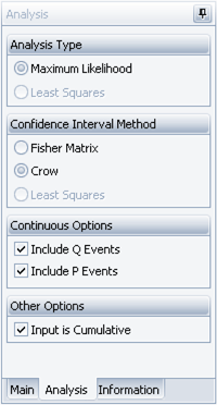
• Q: indicates that the failure was due to a quality issue. An example of this might be a failure caused by a bolt not being tightened down properly. You have the option to decide whether or not to include quality issues in the analysis. This option can be specified by checking or clearing the Include Q Events checkbox under Continuous Options on the Analysis tab, as shown in Figure Q-event options.
• P: indicates that the failure was due to a performance issue. You can determine whether or not to include performance issues in the analysis. This option can be specified by checking or clearing the Include P Events checkbox under Continuous Options on the Analysis tab, as shown in Figure Q-event options.
• AP: indicates an analysis point. Analysis points can be shown in a multi-phase plot to track overall project progress and can be compared to an idealized growth curve.
• PH: indicates the end of a test phase. Test phases can be shown in a multi-phase plot to track overall project progress and can be compared to planned growth phases. RGA 7 allows for a maximum of seven test phases to be defined.
• X: indicates that the data point will be excluded from the analysis. An "X" can be placed in front of any existing event code or entered by itself. This row of data will then not be included in the analysis.

[math]\displaystyle{ }[/math]

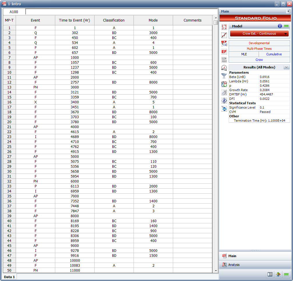
Figure Folioxample shows an example of a Crow Extended - Continuous Evaluation folio with all of the possible event codes. As you can see, each failure is indicated with A, BC or BD in the Classification column. In addition, any text can be used to specify the mode. In this figure, failure codes were used in the Mode column for simplicity, but you could just as easily use Seal Leak, or whatever designation you deem appropriate for the failure mode.

[math]\displaystyle{ }[/math]

Figure 10.1: Options to include or exclude quiality and performance events from the Crow Extended- Continuous Evaluation analysis.

Figure 10.2: A Crow Extended- Continuous Evaluation folio with all possible event codes.

[math]\displaystyle{ p }[/math] Ratio

In the Crow Extended - Continuous evaluation, there is a certain probability of not incorporating a corrective action by time [math]\displaystyle{ T }[/math] . This is the additional (third parameter), as compared to the Crow Extended model. We define [math]\displaystyle{ p }[/math] as:

[math]\displaystyle{ p=\frac{\text{All modes such that, if seen, will be corrected at time }T\text{, or later}}{\text{All failure modes such that, if seen, the corrective action will be delayed}} }[/math]

It is assumed that the ratio [math]\displaystyle{ p }[/math] remains fixed over . This implies that each time a distinct failure mode is seen, the probability that the corrective action is delayed until time [math]\displaystyle{ T }[/math] or later is [math]\displaystyle{ p }[/math] . In other words, each time a new BD mode is seen over [math]\displaystyle{ (0,T) }[/math] there is a probability [math]\displaystyle{ p }[/math] that the corrective action for that mode will not have been incorporated into the system by time [math]\displaystyle{ T }[/math] . Under the Crow Extended two-parameter model, this probability is always equal to 1 at time [math]\displaystyle{ T. }[/math]

Effectiveness Factors

As discussed in Chapter 9, it is very important to note that failure modes are rarely totally eliminated by a corrective action. After failure modes have been found and fixed, a certain percentage of the failure intensity will be removed, but a certain percentage of the failure intensity will also remain. For each BD mode, an effectiveness factor (EF) is required to estimate how effective the corrective action will be in eliminating the failure intensity due to the failure mode. The EF is the fractional decrease in a mode's failure intensity after a corrective action has been made and must be a value between 0 and 1. A study on EFs showed that an average EF, [math]\displaystyle{ d, }[/math] was about [math]\displaystyle{ 0.7 }[/math] . However, individual EFs for the failure modes may be larger or smaller than the average. Therefore, typically about [math]\displaystyle{ 30% }[/math] , i.e. [math]\displaystyle{ 100(1-d)% }[/math] , of the BD mode failure intensity will remain in the system after all of the corrective actions have been implemented.
Similar to the Crow Extended model, each BD mode has an effectiveness factor that represents the decrease in failure intensity for that mode once the corrective action has been incorporated into the system. In addition, a delayed fix can be incorporated any time after the first occurrence of the failure mode. Therefore, delayed fixes can be incorporated before the end of the test phase, at the end of the test phase (just like the Crow Extended delayed fixes) or not incorporated at all at the end of the current test phase but postponed for a subsequent test phase. For calculation purposes, any delayed fixes that are incorporated during the test (those with an I event code) do not need to have an effectiveness factor specified, since the fix is already incorporated in the system. Figure EF shows how effectiveness factors are defined in the Crow Extended - Continuous Evaluation model in RGA 7. The figure also shows that you can specify if the delayed fix was actually implemented at the end of the current test phase, at a later phase or not implemented at all.

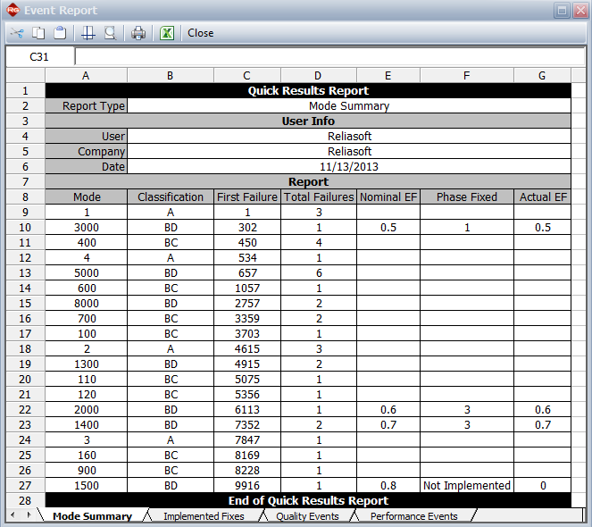
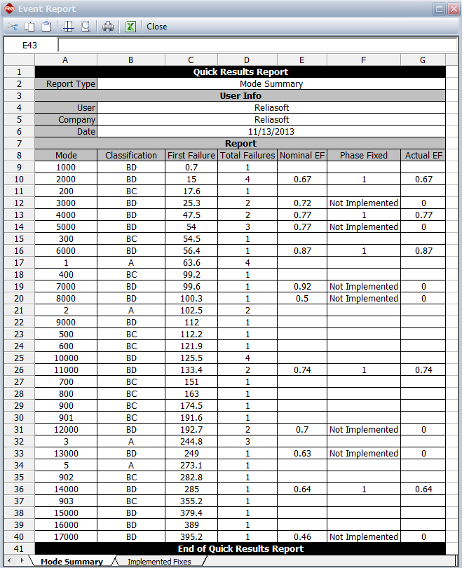
For a Type BD failure mode not yet corrected but still deferred, the Actual Effectiveness Factor for that mode is zero. The Actual Effectiveness Factor for a deferred Type BD failure mode will stay at zero until the point when the corrective action will be incorporated. At that time, the Actual Effectiveness Factor is changed to equal the Assigned Effectiveness Factor for that mode. At this point, the Nominal Effectiveness Factor (the effectiveness factor assuming fixes are implemented at the end of the specific phase) and the Actual Effectiveness Factor are the same. In other words, if a fix is not incorporated for a BD mode, its actual effectiveness for reducing failure intensity is zero, and the assigned effectiveness factor will be used only for projecting the MTBF (or failure intensity), as it will be discussed in Section 10.2.5. Figure Event report shows an event report in RGA 7. At the end of the test phase, depending on whether the BD mode was specified as fixed or not fixed, the actual EF is zero (e.g. mode BD3000) or equal to the nominal EF (e.g. mode BD1500).

[math]\displaystyle{ }[/math]

Figure 10.3: Effectiveness factors defined for each unique BD mode not corrected during the test. If the fix will be impletmented at the end of a test phase, the phase number is indicated.

The Average Nominal EF is:

[math]\displaystyle{ {{d}_{N}}=\frac{\underset{i=1}{\overset{M}{\mathop{\sum }}}\,{{d}_{Ni}}}{M} }[/math]

where [math]\displaystyle{ M }[/math] is the total number of open and distinct BD modes at time [math]\displaystyle{ {{T}_{J}} }[/math] and is the Nominal Effectiveness Factor as specified for each of the BD mode.
The Average Actual EF is:

[math]\displaystyle{ {{d}_{A}}=\frac{\underset{i=1}{\overset{M}{\mathop{\sum }}}\,{{d}_{Ai}}}{M} }[/math]

where [math]\displaystyle{ M }[/math] is the total number of open and distinct BD modes at time [math]\displaystyle{ {{T}_{J}} }[/math] and [math]\displaystyle{ {{d}_{{{A}_{i}}}} }[/math] is the Actual Effectiveness Factor at time [math]\displaystyle{ {{T}_{j}} }[/math] for each BD mode.

Figure 10.4: Event report showing nominal and actual effectiveness factors.

Growth Potential and Projections

The failure intensity left in the system will depend on the management strategy that determines the classification of the A, BC and BD failure modes. The engineering effort applied to the corrective actions determines the effectiveness factors. In addition, the failure intensity depends on [math]\displaystyle{ h(t) }[/math] , which is the rate at which unique BD failure modes are being discovered during testing. The rate of discovery drives the opportunity to take corrective actions based on the seen failure modes and it is an important factor in the overall reliability growth rate. The reliability growth potential is the limiting value of the failure intensity as time [math]\displaystyle{ T }[/math] increases. This limit is the maximum MTBF that can be attained with the current management strategy. The maximum MTBF will be attained when all BD modes have been observed and fixed.
If all seen BD modes are corrected by time [math]\displaystyle{ T }[/math] , that is, no deferred corrective actions at time [math]\displaystyle{ T }[/math] , then the Growth Potential is the maximum attainable based on the Type BD designation of the failure modes, the corresponding assigned effectiveness factors and the remaining A modes in the system. This is called the Nominal Growth Potential. If some seen BD modes are not corrected at the end of the current test phase then the prevailing growth potential is below the maximum attainable with the Type BD designation of the failure modes and the corresponding assigned effectiveness factors. The Crow-AMSAA (NHPP) model is used to estimate the current demonstrated MTBF or [math]\displaystyle{ MTB{{F}_{D}}. }[/math] The demonstrated MTBF does not take into account any type of projected improvements. Refer to Chapter 5 for more details on the Crow-AMSAA (NHPP) model. The corresponding current demonstrated failure intensity is:

[math]\displaystyle{ {{\lambda }_{D}}=\lambda \beta {{T}^{\beta -1}} }[/math]

or:

[math]\displaystyle{ {{\lambda }_{D}}=\frac{1}{MTB{{F}_{D}}} }[/math]

The nominal growth potential factor is:

[math]\displaystyle{ {{\lambda }_{NGPFactor}}=\underset{i=1}{\overset{M}{\mathop \sum }}\,\left( 1-{{d}_{Ni}} \right)\frac{{{N}_{i}}}{T} }[/math]

where:
• [math]\displaystyle{ M }[/math] is the total number of distinct unfixed BD modes at time [math]\displaystyle{ {{T}_{j}} }[/math] .
• [math]\displaystyle{ {{d}_{Ni}} }[/math] is the assigned (nominal) EF for the [math]\displaystyle{ {{i}^{th}} }[/math] unfixed BD mode at time [math]\displaystyle{ {{T}_{j}}. }[/math]
• [math]\displaystyle{ {{N}_{i}} }[/math] is the total number of failures over (0, [math]\displaystyle{ {{T}_{j}} }[/math] ) for the distinct unfixed BD mode [math]\displaystyle{ i }[/math] . The nominal growth potential factor signifies the failure intensity of the [math]\displaystyle{ M }[/math] modes after corrective actions have been implemented for them, using the nominal values for the effectiveness factors.
Similarly, the actual growth potential factor is:

[math]\displaystyle{ {{\lambda }_{AGPFactor}}=\underset{i=1}{\overset{M}{\mathop \sum }}\,\left( 1-{{d}_{Ai}} \right)\frac{{{N}_{i}}}{T} }[/math]

where [math]\displaystyle{ {{d}_{Ai}} }[/math] is the actual EF for the [math]\displaystyle{ {{i}^{th}} }[/math] unfixed BD mode at time [math]\displaystyle{ {{T}_{j}}. }[/math]
The actual growth potential factor signifies the failure intensity of the [math]\displaystyle{ M }[/math] modes after corrective actions have been implemented for them, using the actual values for the effectiveness factors.
Based on the definition of BD modes for the Crow Extended - Continuous Evaluation model, the estimate of [math]\displaystyle{ p }[/math] at time [math]\displaystyle{ {{T}_{j\text{ }}} }[/math] is calculated as follows:

[math]\displaystyle{ p=\frac{\text{Total number of distinct unfixed BD modes at time }{{T}_{j}}}{\text{Total number of distinct BD modes at time }{{T}_{j}}\text{ (both fixed and unfixed)}} }[/math]

The unfixed BD mode failure intensity at time [math]\displaystyle{ {{T}_{j}} }[/math] is:

[math]\displaystyle{ \lambda_{BD\text{unfixed}} = \frac{\text{Total number of unfixed BD failures at time T_j}}{T_j} }[/math]

Similar to the Crow Extended model, the discovery function at time [math]\displaystyle{ T }[/math] for the Crow Extended - Continuous Evaluation model is calculated using all the first occurrences of the all the BD modes, both fixed and unfixed. [math]\displaystyle{ h(t) }[/math] is the unseen BD mode failure intensity and is also the rate at which new unique BD modes are being discovered.

[math]\displaystyle{ \begin{align} & \widehat{h}(T|BD)= & {{\widehat{\lambda }}_{BD}}{{\widehat{\beta }}_{BD}}{{T}^{{{\widehat{\beta }}_{BD}}-1}} \\ & = & \frac{M{{\widehat{\beta }}_{BD}}}{T} \end{align} }[/math]

where:
• [math]\displaystyle{ {{\widehat{\beta }}_{BD}} }[/math] is the unbiased estimated of [math]\displaystyle{ \beta }[/math] for the Crow-AMSAA (NHPP) model based on the first occurrence of [math]\displaystyle{ M }[/math] distinct BD modes.
• [math]\displaystyle{ {{\widehat{\lambda }}_{BD}} }[/math] is the unbiased estimated of [math]\displaystyle{ \lambda }[/math] for the Crow-AMSAA (NHPP) model based on the first occurrence of [math]\displaystyle{ M }[/math] distinct BD modes.
[math]\displaystyle{ {{\widehat{\beta }}_{BD}} }[/math] and [math]\displaystyle{ {{\widehat{\lambda }}_{BD}} }[/math] are also known as the Rate of Discovery Parameters.
The nominal growth potential failure intensity is:

[math]\displaystyle{ \lambda_{NGP} = \lambda_D - \lambda_{BD\text{unfixed}} + \lambda_{NGP\text{Factor}} + d_N\cdot p\cdot h(T) - d_N h(T) }[/math]

and the nominal growth potential MTBF is:

[math]\displaystyle{ MTB{{F}_{NGP}}=\frac{1}{{{\lambda }_{NGP}}} }[/math]

The nominal projected failure intensity at time [math]\displaystyle{ T }[/math] is:

[math]\displaystyle{ {{\lambda }_{NP}}={{\lambda }_{NGP}}+{{d}_{N}}h(T) }[/math]

and the nominal projected MTBF at time [math]\displaystyle{ T }[/math] is:

[math]\displaystyle{ MTB{{F}_{NP}}=\frac{1}{{{\lambda }_{NP}}} }[/math]

The actual growth potential failure intensity is:

[math]\displaystyle{ \lambda{AGP} = \lambda_D - \lambda_{BD\text{unfixed}} + \lambda{AGP\text{Factor} + d_A\cdot p\cdot h(T) - d_A h(T)} }[/math]

and the actual growth potential MTBF is:

[math]\displaystyle{ MTB{{F}_{AGP}}=\frac{1}{{{\lambda }_{AGP}}} }[/math]

The actual projected failure intensity at time is:

[math]\displaystyle{ {{\lambda }_{AP}}={{\lambda }_{AGP}}+{{d}_{A}}\cdot h\left( T \right) }[/math]

and the actual projected MTBF at time is:

[math]\displaystyle{ MTB{{F}_{AP}}=\frac{1}{{{\lambda }_{AP}}} }[/math]

In terms of confidence intervals and goodness-of-fit tests, the calculations are the same as for the Crow Extended model, described in Chapter 9.

Example 1

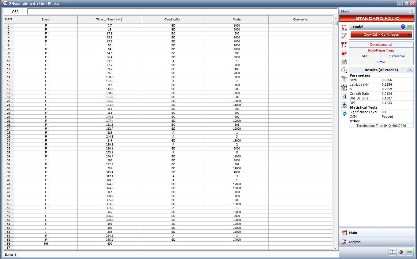
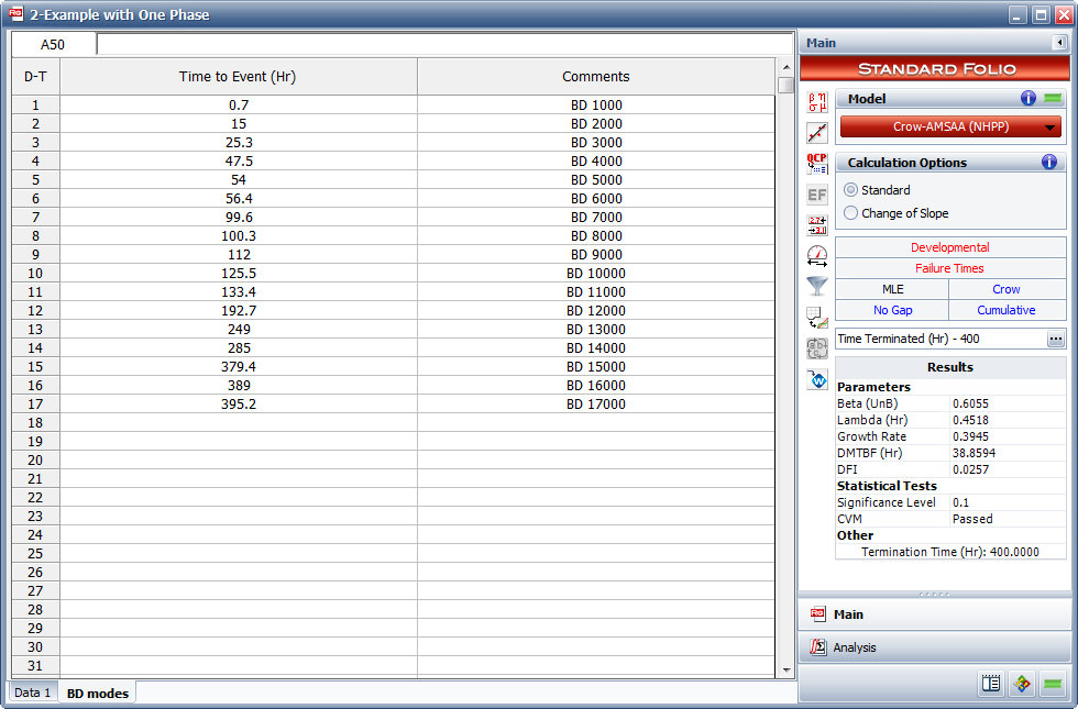
Table 10.2 shows the Multi-Phase data with failure and fix implementation events. Figure Example 1 data in RGA 7 shows the Table 10.2 data as entered in RGA 7. Note that since this is a time terminated test with a single phase ending at [math]\displaystyle{ T=400 }[/math] , the last event entry is a phase (PH) with time to event = 400.

Table 10.2 - Multi-Phase data for a time terminated test at [math]\displaystyle{ T=400 }[/math]

Event	Time to Event	Classification	Mode		Event	Time to Event	Classification	Mode
F	0.7	BD	1000		F	244.8	A	3
F	15	BD	2000		F	249	BD	13000
F	17.6	BC	200		F	250.8	A	2
F	25.3	BD	3000		F	260.1	BD	2000
F	47.5	BD	4000		F	273.1	A	5
I	50	BD	1000		F	274.7	BD	11000
F	54	BD	5000		I	280	BD	9000
F	54.5	BC	300		F	282.8	BC	902
F	56.4	BD	6000		F	285	BD	14000
F	63.6	A	1		F	315.4	BD	4000
F	72.2	BD	5000		F	317.1	A	3
F	99.2	BC	400		F	320.6	A	1
F	99.6	BD	7000		F	324.5	BD	12000
F	100.3	BD	8000		F	324.9	BD	10000
F	102.5	A	2		F	342	BD	5000
F	112	BD	9000		F	350.2	BD	3000
F	112.2	BC	500		F	355.2	BC	903
F	120.9	BD	2000		F	364.6	BD	10000
F	121.9	BC	600		F	364.9	A	1
F	125.5	BD	10000		I	365	BD	10000
F	133.4	BD	11000		F	366.3	BD	2000
F	151	BC	700		F	379.4	BD	15000
F	163	BC	800		F	389	BD	16000
F	174.5	BC	900		I	390	BD	15000
F	177.4	BD	10000		I	393	BD	16000
F	191.6	BC	901		F	394.9	A	3
F	192.7	BD	12000		F	395.2	BD	17000
F	213	A	1

Figure EF example 1 shows the effectiveness factors for the unfixed BD modes and information concerning whether the fix will be implemented. Since we have only one test phase for this example, a 1 indicates that the fix will be implemented at the end of the first (and only) phase.
[math]\displaystyle{ }[/math]

Figure 10.5: Example 1 data in RGA 7.

Do the following:
1) Determine the current demonstrated MTBF and failure intensity at time [math]\displaystyle{ T }[/math] .
2) Determine the nominal and actual average effectiveness factor at time [math]\displaystyle{ T }[/math] .
3) Determine the ratio.
4) Determine the nominal and actual growth potential factor.
5) Determine the unfixed BD mode failure intensity at time [math]\displaystyle{ T. }[/math]
6) Determine the rate of discovery parameters and the rate of discovery function at time [math]\displaystyle{ T }[/math] .
7) Determine the nominal growth potential failure intensity and MTBF at time [math]\displaystyle{ T. }[/math]
8) Determine the nominal projected failure intensity and MTBF at time [math]\displaystyle{ T. }[/math]
9) Determine the actual growth potential failure intensity and MTBF at time [math]\displaystyle{ T. }[/math]
10) Determine the actual projected failure intensity and MTBF at time [math]\displaystyle{ T. }[/math]

Solution
1) As seen in Chapter 5, for a time terminated test, [math]\displaystyle{ \beta }[/math] is estimated by the following equation:

[math]\displaystyle{ \widehat{\beta }=\frac{n}{n\ln {{T}^{*}}-\underset{i=1}{\overset{n}{\mathop{\sum }}}\,\ln {{T}_{i}}} }[/math]

where in this case [math]\displaystyle{ {{T}^{*}}= }[/math] termination time [math]\displaystyle{ =400, }[/math] and [math]\displaystyle{ n }[/math] is the total number of failures. In this example [math]\displaystyle{ n=50 }[/math] . Note that there are five fix implementation events and one event that marks the end of the phase. These should not be counted as failures.
So in this case we find that [math]\displaystyle{ \beta =0.9866. }[/math]
Note that here we calculated the biased estimate of [math]\displaystyle{ \beta }[/math] but we could have used the unbiased estimate as presented in Chapter 5. The choice of calculating the biased or unbiased estimate of [math]\displaystyle{ \beta }[/math] can be set in the User Setup in RGA 7.
Then solve for [math]\displaystyle{ \lambda , }[/math] based on the Crow-AMSAA (NHPP) equation explained in Chapter 5, Section 5.1.1:

[math]\displaystyle{ \begin{align} & \widehat{\lambda }= & \frac{n}{{{T}^{*\beta }}} \\ & = & \frac{50}{{{400}^{0.9866}}} \\ & = & 0.1354 \end{align} }[/math]

The demonstrated MTBF of the system at time [math]\displaystyle{ T=400 }[/math] is:

[math]\displaystyle{ \begin{align} & MTB{{F}_{D}}= & \frac{1}{\lambda \beta {{T}^{\beta -1}}} \\ & = & 8.1087 \end{align} }[/math]

The corresponding current demonstrated failure intensity is:

[math]\displaystyle{ \begin{align} & {{\lambda }_{D}}= & \frac{1}{MTB{{F}_{D}}} \\ & = & 0.1233 \end{align} }[/math]

2) The average nominal effectiveness factor at time [math]\displaystyle{ T }[/math] is given by Eqn. (Average Nominal EF):

[math]\displaystyle{ \begin{align} & {{d}_{N}}= & \frac{\underset{i=1}{\overset{M}{\mathop{\sum }}}\,{{d}_{Ni}}}{M} \\ & = & \frac{0.67+0.72+0.77+0.77+0.87+0.92+0.5+0.74+0.7+0.63+0.64+0.46}{12} \\ & = & 0.6992 \end{align} }[/math]

The average actual effectiveness factor at time [math]\displaystyle{ T }[/math] is given by Eqn. (Average actual EF):

[math]\displaystyle{ \begin{align} & {{d}_{A}}= & \frac{\underset{i=1}{\overset{M}{\mathop{\sum }}}\,{{d}_{Ai}}}{M} \\ & = & \frac{0.67+0+0.77+0+0.87+0+0+0.74+0+0+0.64+0}{12} \\ & = & 0.3075 \end{align} }[/math]

3) The [math]\displaystyle{ p }[/math] ratio is calculated by using Eqn. (p ratio):

[math]\displaystyle{ \begin{align} & p= & \frac{\text{Total number of distinct unfixed BD modes at time }400}{\text{Total number of distinct BD modes at time }400\text{ (both fixed and unfixed)}} \\ & = & \frac{12}{12+5} \\ & = & 0.7059 \end{align} }[/math]

4) The nominal growth potential factor is given by Eqn. (Nonimal GP Factor) :

[math]\displaystyle{ {{\lambda }_{NGPFactor}}=\underset{i=1}{\overset{M}{\mathop \sum }}\,\left( 1-{{d}_{Ni}} \right)\frac{{{N}_{i}}}{T} }[/math]

The total number [math]\displaystyle{ M }[/math] of distinct unfixed BD modes at time [math]\displaystyle{ 400 }[/math] is [math]\displaystyle{ M=12. }[/math]

[math]\displaystyle{ {{d}_{Ni}} }[/math] is the assigned (nominal) EF for the [math]\displaystyle{ {{i}^{th}} }[/math] unfixed BD mode at time [math]\displaystyle{ {{T}_{j}}, }[/math] (as given in Figure EF example 1).

[math]\displaystyle{ {{N}_{i}} }[/math] is the total number of failures over (0, [math]\displaystyle{ 400 }[/math] ) for the distinct unfixed BD mode [math]\displaystyle{ i }[/math] . This is summarized in Table 10.3.

Table 10.3 - Number of failures for unfixed BD modes

Classification	Mode	Number of Failures
BD	2000	4
BD	3000	2
BD	4000	2
BD	5000	3
BD	6000	1
BD	7000	1
BD	8000	1
BD	11000	2
BD	12000	2
BD	13000	1
BD	14000	1
BD	17000	1
		Sum = 21

Based on the above, the nominal growth potential factor is calculated as:

[math]\displaystyle{ {{\lambda }_{NGPFactor}}=0.0153 }[/math]

The actual growth potential factor is given by Eqn. (Actual GP factor):

[math]\displaystyle{ {{\lambda }_{AGPFactor}}=\underset{i=1}{\overset{M}{\mathop \sum }}\,\left( 1-{{d}_{Ai}} \right)\frac{{{N}_{i}}}{T} }[/math]

where [math]\displaystyle{ {{d}_{Ai}} }[/math] is the actual EF for the [math]\displaystyle{ {{i}^{th}} }[/math] unfixed BD mode at time 400, depending on whether a fix was implemented at time 400 or not. Figure Event report example 1 shows an event report from RGA 7 where it can be seen that the actual EF is zero if a fix was not implemented at 400, or equal to the nominal EF if the fix was implemented at 400.

[math]\displaystyle{ }[/math]

Figure 10.7: Event report for Example 1.

Based on the above, the actual growth potential factor is calculated as:

[math]\displaystyle{ {{\lambda }_{AGPFactor}}=0.0344 }[/math]

5) The total number of unfixed BD modes is 21, based on Table 10.2. From Eqn. (lambdaBDunfixed), the unfixed BD mode failure intensity at time [math]\displaystyle{ 400 }[/math] is:

6) The discovery rate parameters at time [math]\displaystyle{ 400 }[/math] are calculated using all the first occurrences of all the BD modes, both fixed and unfixed. [math]\displaystyle{ {{\widehat{\beta }}_{BD}} }[/math] is the unbiased estimated of [math]\displaystyle{ \beta }[/math] for the Crow-AMSAA (NHPP) model based on the first occurrence of the 17 distinct BD modes in our example. [math]\displaystyle{ {{\widehat{\lambda }}_{BD}} }[/math] is the unbiased estimate of [math]\displaystyle{ \lambda }[/math] for the Crow-AMSAA (NHPP) model based on the first occurrence of the [math]\displaystyle{ 17 }[/math] distinct BD modes. Figure first occurence BD shows the first time to failure for each of the 17 distinct modes and the results of the analysis using the Crow-AMSAA (NHPP) model in RGA 7 (note that the calculation settings in the User Setup have to be set to calculate unbiased [math]\displaystyle{ \beta }[/math] in this case).

So we have:

[math]\displaystyle{ {{\widehat{\beta }}_{BD}}=0.6055 }[/math]

and:

[math]\displaystyle{ {{\widehat{\lambda }}_{BD}}=0.4518 }[/math]

The equations used to determine these parameters have been explained in question 1 of this example and are also presented in detail in Chapter 5, Section 5.1.1.

Based on Eqn. (Discovery Function), the discovery rate function at time 400 is:

[math]\displaystyle{ \begin{align} & \widehat{h}(T|BD)= & {{\widehat{\lambda }}_{BD}}{{\widehat{\beta }}_{BD}}{{T}^{{{\widehat{\beta }}_{BD}}-1}} \\ & = & 0.4518\cdot 0.6055\cdot {{400}^{0.6055-1}} \\ & = & 0.0257 \end{align} }[/math]

This is the failure intensity of the unseen BD modes at time 400. In this case, it means that 0.0257 new BD modes are discovered per hour, or one new BD mode is discovered every 38.9 hours.

Figure 10.8: Furst occurrence of each BD mode.

Based on Eqn. (Nominal Growth Potential failure intensity), the nominal growth potential failure intensity is:

This is the minimum attainable failure intensity if all delayed corrective actions are implemented for the modes that have been seen and delayed corrective actions are also implemented for the unseen BD modes, assuming testing would continue until all unseen BD modes are revealed.
From Eqn. (Nominal Growth Potential MTBF), the nominal growth potential MTBF is:

[math]\displaystyle{ \begin{align} & MTB{{F}_{NGP}}= & \frac{1}{{{\lambda }_{NGP}}} \\ & = & \frac{1}{0.080} \\ & = & 12.37 \end{align} }[/math]

This is the maximum attainable MTBF if all delayed corrective actions are implemented for the modes that have been seen and delayed corrective actions are also implemented for the unseen BD modes, assuming testing would continue until all unseen BD modes are revealed.

8) From Eqn. (Nominal projected failure intensity), the nominal projected failure intensity at time [math]\displaystyle{ 400 }[/math] is:

[math]\displaystyle{ \begin{align} & {{\lambda }_{NP}}= & {{\lambda }_{NGP}}+{{d}_{N}}h(400) \\ & = & 0.080+0.6992\cdot 0.0257 \\ & = & 0.0988 \end{align} }[/math]

This is the projected failure intensity assuming all delayed fixes have been implemented for the modes that have been seen. The nominal projected MTBF at time [math]\displaystyle{ 400 }[/math] is:

[math]\displaystyle{ \begin{align} & MTB{{F}_{NP}}= & \frac{1}{{{\lambda }_{NP}}} \\ & = & \frac{1}{0.0988} \\ & = & 10.11 \end{align} }[/math]

This is the projected MTBF assuming all delayed fixes have been implemented for the modes that have been seen.
9) Based on Eqn. (Actual GP FI), the actual growth potential failure intensity is:

This is the minimum attainable failure intensity based on the current management strategy.

The actual growth potential MTBF is:

[math]\displaystyle{ \begin{align} & MTB{{F}_{AGP}}= & \frac{1}{{{\lambda }_{AGP}}} \\ & = & \frac{1}{0.1029} \\ & = & 9.71 \end{align} }[/math]

This is the maximum attainable MTBF based on the current management strategy.
10) From Eqn. (Actual projected FI), the actual projected failure intensity at time is:

[math]\displaystyle{ \begin{align} & {{\lambda }_{AP}}= & {{\lambda }_{AGP}}+{{d}_{A}}\cdot h\left( 400 \right) \\ & = & 0.1029+0.3075\cdot 0.0257 \\ & = & 0.1108 \end{align} }[/math]

This is the projected failure intensity based on the current management strategy.
The actual projected MTBF at time is:

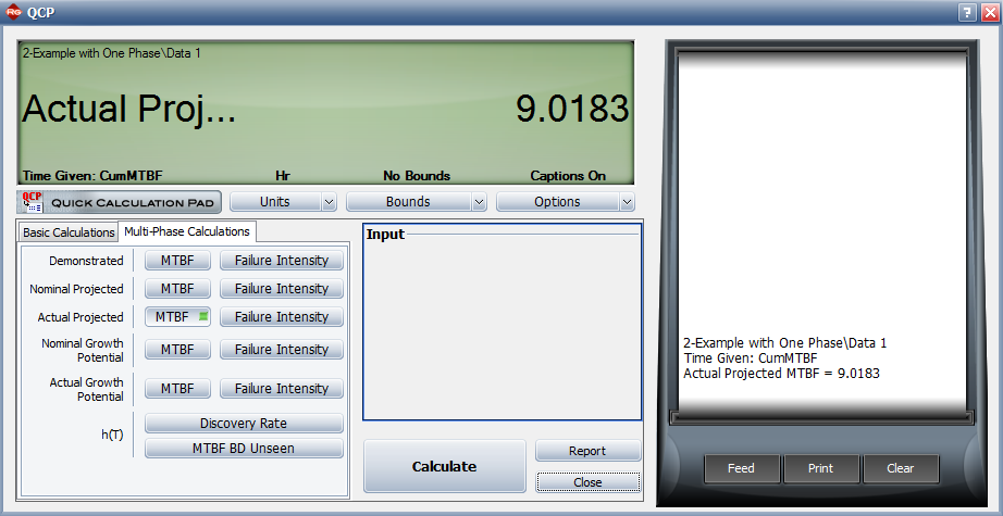
[math]\displaystyle{ \begin{align} & MTB{{F}_{AP}}= & \frac{1}{{{\lambda }_{AP}}} \\ & = & \frac{1}{0.1108} \\ & = & 9.01 \end{align} }[/math]

This is the projected MTBF based on the current management strategy. Figure QCP MTBFac demonstrates how we can derive the results of this example by using RGA 7's Quick Calculation Pad (QCP). Here we chose to calculate the actual projected MTBF.

Figure 10.9: Multi-Phase calculations using the QCP.

Example 2

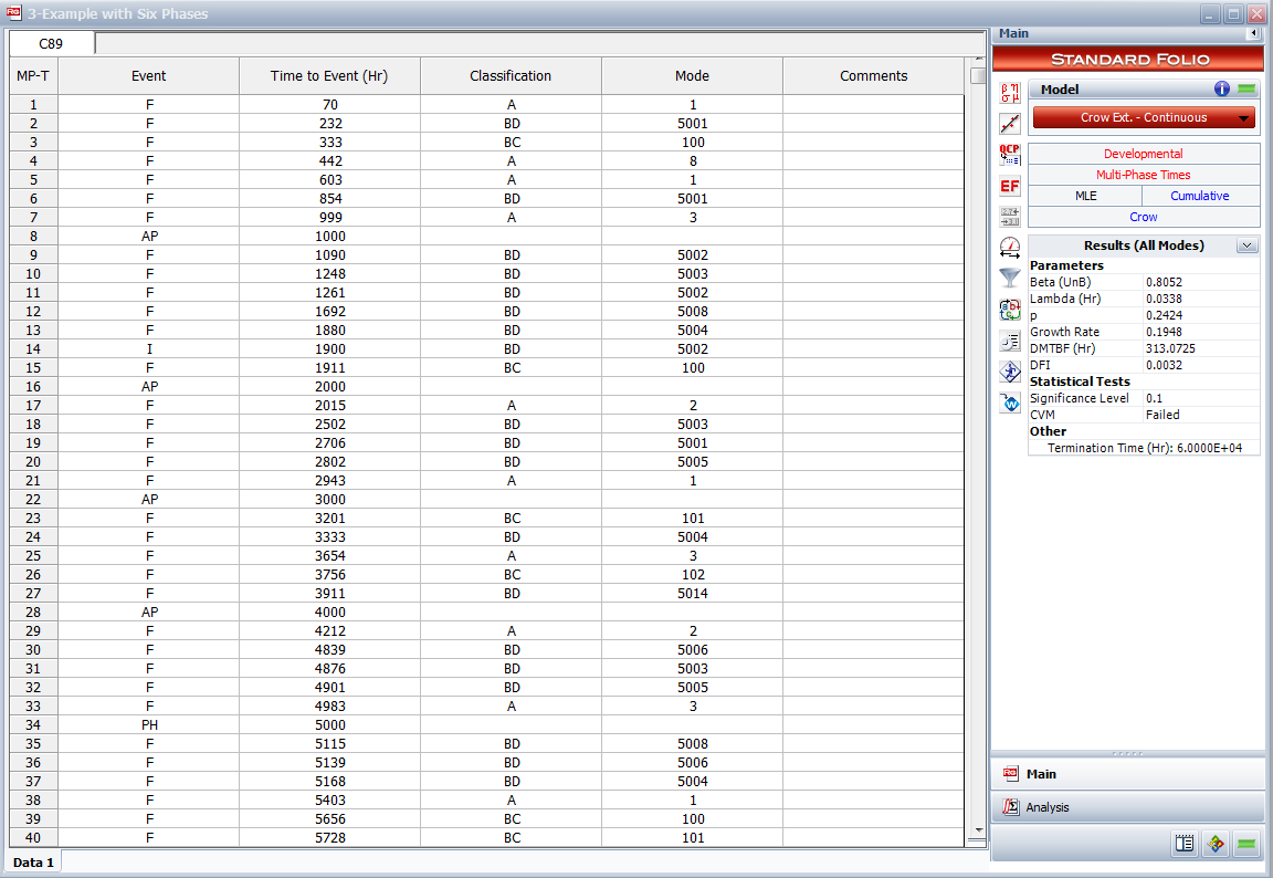
The Crow Extended - Continuous Evaluation model allows data analysis across multiple phases, up to seven individual phases. Figure Example2table, 6 phases shows a portion of failure time test results obtained across six phases. Analysis points are specified for continuous evaluation every 1000 hours. The cumulative test times at the end of each test phase are 5000, 15000, 25000, 35000, 45000 and 60000 hours.

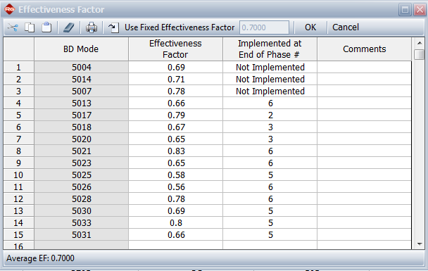
Figure EFxample2 shows the effectiveness factors for the BD modes that do not have an associated fix implementation event. In other words, these are unfixed BD modes. Note that this specifies the phase after which the BD mode will be fixed, if any.

[math]\displaystyle{ }[/math]

Figure 10.10: Portion of test results for a six-phase reliability growth test program.

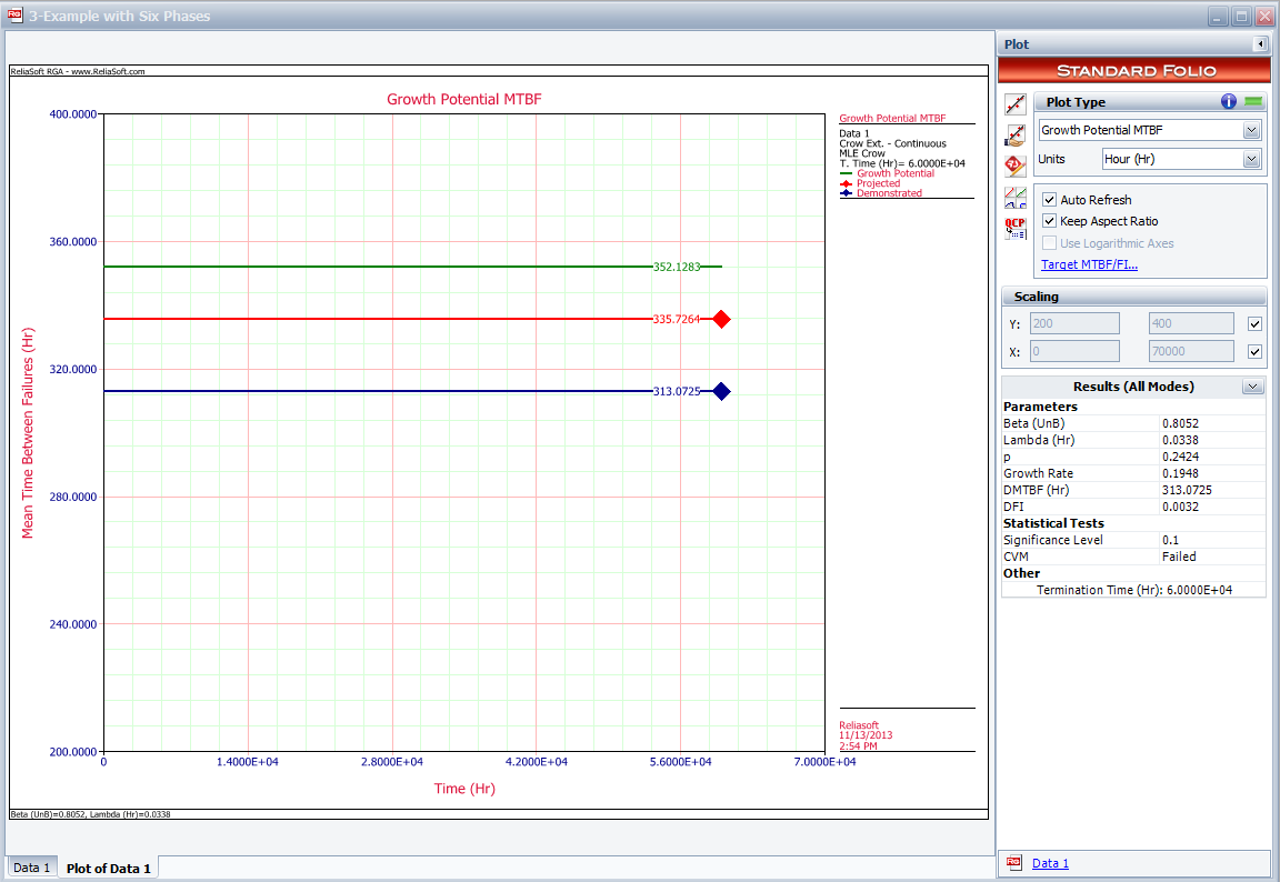
Figure Example2Plot shows the overall test results in terms of demonstrated, projected and growth potential MTBF.

[math]\displaystyle{ }[/math]

Figure 10.11: Effectiveness factor and phase of implementation for the BD failure modes that were not fixed during a test phase (I events).

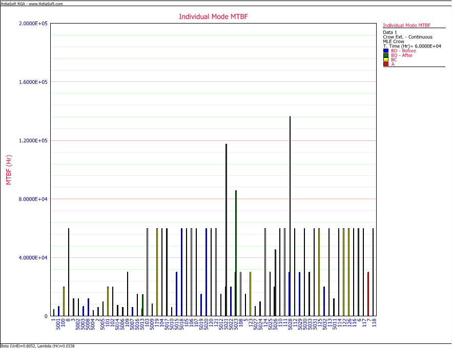
Figure Indivdual Mode MTBF shows the Before and After MTBFs for all the individual modes. Note that the After MTBFs are calculated by taking into account the respective effectiveness factors for each of the unfixed BD modes.

[math]\displaystyle{ }[/math]

Figure 10.12: Demonstrated, projected and growth potential MTBF for the six-phase test program.

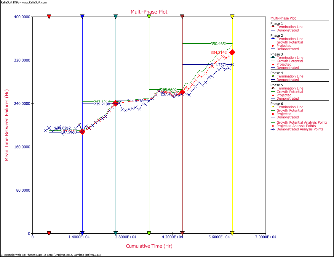
The analysis points are used to track overall growth inside and across phases, at desired intervals. A multi-phase plot can be created by right-clicking Additional Plots in the Project Explorer and selecting Add MultiPhase Plot. The MultiPhase Plot Wizard guides you through the process concerning the data sheet selection. Since the Crow Extended - Continuous Evaluation was used for the six-phase test, we select the Multi-Phase option. A Multi-Phase data sheet can be associated with the multi-phase plot. Also, if there is an existing Planning folio, the multi-phase plot can bring the test results together with the Planning. This allows you to track the overall reliability program against the goals and set plans at each stage of the test. Additional information on combining a Planning folio and a MultiPhase plot is presented in Chapter 11.

Figure Multi-phase plot shows the multi-phase plot for the six phases of the reliability growth test program. This plot can be a powerful tool for overall tracking of the reliability growth program. It displays the termination time for each phase of testing along with the demonstrated, projected and growth potential MTBFs at those times. The plot also displays these calculated MTBFs at specified analysis points, which are determined based on the "AP" events in the data sheet.

[math]\displaystyle{ }[/math]

Figure 10.13: Individual mode MTBF plot for the six-phase test program.

Figure 10.14: Multi-phase plot with analysis points and phases for the six-phase test.

Discrete Data

The Crow Extended - Continuous Evaluation model also can be applied for discrete data from one-shot (success/failure) testing. In RGA 7, the Multi-Phase > Mixed Data option gives a data sheet that can accommodate data from tests where a single unit is tested for each successive configuration (individual trial-by-trial), where multiple units are tested for each successive configuration (configurations in groups) or a combination of both. Corrective actions cannot take place at the time of failure for discrete data. With that in mind, the mixed data type does not allow for BC modes. The delayed corrective actions over time can be either fixed or unfixed, based on a subsequent implementation (I) event. So, for discrete data there are only unfixed BD modes or fixed BD modes. As a practical application, think of a multi-phase program for missile systems. Since these are one-shot items, the fixes to failure modes are delayed until at least the next trial. Note that for calculation purposes it is required to have at least three failures in the first interval. If that is not the case, then the data set needs to be grouped until this requirement is met before calculating. RGA 7 performs this operation in the background.

Example 3

A one-shot system underwent reliability growth development for a total of 20 trials. The test was performed as a combination of configuration in groups and individual trial-by-trial. Table 10.4 shows the obtained data set. The "Failures in Interval" column specifies the number of failures that occurred in each interval and the "Cumulative Trials" column specifies the cumulative number of trials at the end of that interval.

The table also gives the classifications of the failure modes. There are 5 BD modes. Of these 5 modes, 2 are corrected during the test (BD3 and BD4) and 3 have not been corrected by time [math]\displaystyle{ T=20 }[/math] (BD1, BD2 and BD5). Do the following: 1) Calculate the parameters of the Crow Extended - Continuous Evaluation model. 2) Calculated the demonstrated reliability at the end of the test. 3) Calculate parameter [math]\displaystyle{ p }[/math] . 4) Calculate the unfixed BD mode failure probability. 5) Calculate the nominal growth potential factor. 6) Calculate the nominal average effectiveness factor. 7) Calculate the discovery failure intensity function at the end of the test. 8) Calculate the nominal projected reliability at the end of the test. 9) Calculate the nominal growth potential reliability at the end of the test. Solution 1) Figure MIxed data shows the data for Example 3 as entered in RGA 7.

The parameters [math]\displaystyle{ \beta }[/math] and [math]\displaystyle{ \lambda }[/math] are calculated as follows (the calculations for these parameters are presented in detail in Chapter 5, Section 5.1.1):

[math]\displaystyle{ \widehat{\beta }=0.8572 }[/math]

and:

[math]\displaystyle{ \widehat{\lambda }=0.4602 }[/math]

2) The corresponding demonstrated unreliability is calculated as: 3) 4) [math]\displaystyle{ {{f}_{D}}=\lambda \beta {{T}^{\beta -1}},\text{with }T\gt 0,\text{ }\lambda \gt 0\text{ and }\beta \gt 0 }[/math] 5) 6) Using the above parameter estimates, the instantaneous unreliability at the end of the test (or [math]\displaystyle{ T=20) }[/math] is equal to:

[math]\displaystyle{ {{f}_{D}}(20)=0.8572\cdot 0.4602\cdot {{20}^{0.8572-1}}=0.2572 }[/math]

The demonstrated reliability is:

[math]\displaystyle{ \begin{align} & {{R}_{D}}= & 1-{{f}_{D}} \\ & = & 1-0.2572=0.7428 \end{align} }[/math]

Note that in discrete data, we calculate reliability and not MTBF, since we are dealing with number of trials and not test time. 7) Assume that the following effectiveness factors are assigned to the unfixed BD modes:

[math]\displaystyle{ \begin{matrix} \text{Classification} & \text{Mode} & \text{Effectiveness Factor} & \text{Implemented at End of Phase} \\ \text{BD} & \text{1} & \text{0}\text{.65} & \text{Phase 1} \\ \text{BD} & \text{2} & \text{0}\text{.70} & \text{Phase 1} \\ \text{BD} & \text{5} & \text{0}\text{.75} & \text{Phase 1} \\ \end{matrix} }[/math]

The parameter [math]\displaystyle{ p }[/math] is the total number of distinct unfixed BD modes at time [math]\displaystyle{ T }[/math] divided by the total number of distinct BD (fixed and unfixed) modes. In this example:

[math]\displaystyle{ p=\frac{3}{5}=0.6 }[/math]

8) The unfixed BD mode failure probability at time [math]\displaystyle{ T }[/math] is the total number of unfixed BD failures (classified at time [math]\displaystyle{ T }[/math] ) divided by the total trials. Based on Table 10.4, we have:

9) Based on Eqn. (Nonimal GP Factor), the nominal growth potential factor is:

[math]\displaystyle{ \begin{align} & {{\lambda }_{NGPFactor}}= & \underset{i=1}{\overset{M}{\mathop \sum }}\,\left( 1-{{d}_{i}} \right)\frac{{{N}_{i}}}{T} \\ & = & \left( 1-{{d}_{1}} \right)\frac{{{N}_{1}}}{T}+\left( 1-{{d}_{2}} \right)\frac{{{N}_{2}}}{T}+\left( 1-{{d}_{5}} \right)\frac{{{N}_{5}}}{T} \\ & = & \left( 1-0.65 \right)\frac{1}{20}+\left( 1-0.70 \right)\frac{2}{20}+\left( 1-0.75 \right)\frac{1}{20} \\ & = & 0.06 \end{align} }[/math]

10) Using Eqn. (Average Nominal EF), the nominal average effectiveness factor is: 11) 12) [math]\displaystyle{ \begin{align} 13) & {{d}_{N}}= & \frac{\underset{i=1}{\overset{M}{\mathop{\sum }}}\,{{d}_{Ni}}}{M} \\ 14) & = & \frac{0.65+0.70+0.75}{3} \\ 15) & = & 0.70 16) \end{align} }[/math] 17) 18) 19) Based on Eqn. (Discovery Function), the discovery function at time [math]\displaystyle{ T }[/math] is calculated using all the first occurrences of all the BD modes, both fixed and unfixed. In our example, we calculate [math]\displaystyle{ {{\widehat{\beta }}_{BD}} }[/math] and [math]\displaystyle{ {{\widehat{\lambda }}_{BD}} }[/math] using only the unfixed BD modes and excluding the second occurrence of BD2, which results in the following:

[math]\displaystyle{ {{\widehat{\beta }}_{BD}}=0.6602 }[/math]

and:

[math]\displaystyle{ {{\widehat{\lambda }}_{BD}}=0.6920 }[/math]

So the discovery failure intensity function at time [math]\displaystyle{ T=20 }[/math] is:

[math]\displaystyle{ \begin{align} & \widehat{h}(T|BD)= & {{\widehat{\lambda }}_{BD}}{{\widehat{\beta }}_{BD}}{{T}^{{{\widehat{\beta }}_{BD}}-1}} \\ & = & 0.6920\cdot 0.6602\cdot {{20}^{0.6602-1}} \\ & = & 0.16507 \end{align} }[/math]

Figure Discovery failure prob function shows the plot for the discovery failure intensity function.

[math]\displaystyle{ }[/math]

20) Based on Eqn. (Nominal projected failure intensity), the nominal projected failure probability at time [math]\displaystyle{ T=20 }[/math] is:

[math]\displaystyle{ \begin{align} & {{f}_{NP}}= & {{f}_{NGP}}+{{d}_{N}}h(T) \\ & = & 0.0701+0.7\cdot 0.16507 \\ & = & 0.1865 \end{align} }[/math]

Therefore, the nominal projected reliability is:

[math]\displaystyle{ \begin{align} & {{R}_{P}}= & 1-0.1856= \\ & = & 0.8135 \end{align} }[/math]

21) Based on Eqn. (Nominal Growth Potential failure intensity), the nominal growth potential unreliability is:

Based on the previous calculation for this example, we have:

[math]\displaystyle{ \begin{align} & {{f}_{NGP}}= & 0.2572-0.2+0.06+0.7\cdot 0.6\cdot 0.16507-0.7\cdot 0.16507 \\ & = & 0.0709 \end{align} }[/math]

So the nominal growth potential reliability is:

[math]\displaystyle{ \begin{align} & {{R}_{NGP}}= & 1-0.0709 \\ & = & 0.9291 \end{align} }[/math]

Figure GPplot shows the plot for the instantaneous demonstrated, projected and growth potential reliability.

Statistical Tests for Effectiveness of Corrective Actions Introduction

The purpose of the statistical tests is to explore the effectiveness of corrective actions during or at the end of a phase. Say we have two phases, Phase 1 and Phase 2. Suppose that corrective actions are incorporated during or at the end of Phase 1. The system is then operated during Phase 2. The general question is whether or not the corrective actions have been effective. There are two questions that can be addressed regarding the effectiveness of the corrective actions: Question 1. Is the average failure intensity for Phase 2 statistically less than the average failure intensity for Phase1? Question 2. Is the average failure intensity for Phase 2 statistically less than the Crow-AMSAA (NHPP) instantaneous failure intensity at the end of Phase 1? Average Failure Intensities Test The purpose of this test is to compare the average failure intensity during Phase 2 with the average failure intensity during Phase 1. The average failure intensity for Phase 1 is:

[math]\displaystyle{ {{\overline{r}}_{1}}=\frac{{{N}_{1}}}{{{T}_{1}}} }[/math]

where [math]\displaystyle{ {{T}_{1}} }[/math] is the Phase 1 test time and [math]\displaystyle{ {{N}_{1}} }[/math] is the number of failures during Phase 1.

Similarly, the average failure intensity for Phase 2 is:

[math]\displaystyle{ {{\overline{r}}_{2}}=\frac{{{N}_{2}}}{{{T}_{2}}} }[/math]

where [math]\displaystyle{ {{T}_{2}} }[/math] is the Phase 2 test time and [math]\displaystyle{ {{N}_{2}} }[/math] is the number of failures during Phase 2. The overall test time, [math]\displaystyle{ T }[/math] , is:

[math]\displaystyle{ T={{T}_{1}}+{{T}_{2}} }[/math]

The overall number of failures, [math]\displaystyle{ N }[/math] , is:

[math]\displaystyle{ N={{N}_{1}}+{{N}_{2}} }[/math]

Define [math]\displaystyle{ P }[/math] as:

[math]\displaystyle{ P=\frac{{{T}_{2}}}{T} }[/math]

If the cumulative binomial probability [math]\displaystyle{ B(k;P,N) }[/math] of up to [math]\displaystyle{ {{N}_{2}} }[/math] failures is less than or equal to the statistical significance [math]\displaystyle{ \alpha }[/math] , then the average failure intensity for Phase 2 is statistically less than the average failure intensity for Phase 1 at the specific significance level. The cumulative binomial distribution probability is given by:

[math]\displaystyle{ B(k;P,N)=\underset{f=0}{\overset{k}{\mathop \sum }}\,\left( \begin{matrix} N \\ f \\ \end{matrix} \right){{P}^{f}}{{\left( 1-P \right)}^{N-f}} }[/math]

which gives the probability that the test failures, [math]\displaystyle{ f }[/math] , are less than or equal to the number of allowable failures, or acceptance number [math]\displaystyle{ k }[/math] in [math]\displaystyle{ N }[/math] trials, when each trial has a probability of succeeding of [math]\displaystyle{ P }[/math] . Example 4 Suppose a test is being conducted and is divided into two phases. The test time for the first Phase is [math]\displaystyle{ {{T}_{1}}=27 }[/math] days and the test time for the second phase is [math]\displaystyle{ {{T}_{2}}=18 }[/math] days. The number of failures during Phase 1 is [math]\displaystyle{ {{N}_{1}}=11 }[/math] and the number of failures during Phase 2 is [math]\displaystyle{ {{N}_{2}}=2. }[/math] Using Eqn. (AFI1), the average failure intensity for Phase 1 is:

[math]\displaystyle{ {{\overline{r}}_{1}}=\frac{{{N}_{1}}}{{{T}_{1}}}=\frac{11}{27}=0.4074. }[/math]

Similarly, using Eqn. (AFI2), the average failure intensity for Phase 2 is:

[math]\displaystyle{ {{\overline{r}}_{2}}=\frac{{{N}_{2}}}{T2}=\frac{2}{18}=0.1111 }[/math]

Although the average failure intensities are different, we want to see, if at the 10% statistical significance level, the average failure intensity for Phase 2 is statistically less than the average failure intensity for Phase 1. Solution Concerning the total test time, using Eqn. (T) we have:

[math]\displaystyle{ T={{T}_{1}}+{{T}_{2}}=27+18=45 }[/math]

Using Eqn. (N), the total number of failures is equal to:

[math]\displaystyle{ N={{N}_{1}}+{{N}_{2}}=11+2=13 }[/math]

Then, by using Eqn. (P) we calculate [math]\displaystyle{ P }[/math] as:

[math]\displaystyle{ P=\frac{{{T}_{2}}}{T}=\frac{18}{45}=0.4 }[/math]

Using Eqn. (Cum.Binomial), we have:

[math]\displaystyle{ \begin{align} & B(k;P,N)= & B({{N}_{2}};P,N) \\ & = & \underset{f=0}{\overset{{{N}_{2}}}{\mathop \sum }}\,\left( \begin{matrix} N \\ {{N}_{2}} \\ \end{matrix} \right){{P}^{f}}{{\left( 1-P \right)}^{N-f}} \\ & = & \underset{f=0}{\overset{2}{\mathop \sum }}\,\left( \begin{matrix} 13 \\ f \\ \end{matrix} \right){{0.4}^{f}}{{\left( 1-0.4 \right)}^{13-f}} \\ & = & 0.058 \end{align} }[/math]

Since 0.058 is lower than 0.10, the conclusion is that at the 10% significance level the average failure intensity for Phase 2 is statistically less than the average failure intensity for Phase 1. The conclusion would be different for a different significance level. For example, at the 5% significance level, since 0.058 is not lower than 0.05, we fail to reject the null hypothesis. In other words, we cannot statistically prove any significant difference between the average failure intensities at the 5% level. Average vs. Demonstrated Failure Intensities Test The purpose of this test is to compare the average failure intensity during Phase 2 with the Crow-AMSAA (NHPP) instantaneous failure intensity at the end of Phase 1; in other words, the demonstrated failure intensity at the end of Phase 1. Once again, the average failure intensity for Phase 2 is given by Eqn. (AFI2):

[math]\displaystyle{ {{\overline{r}}_{2}}=\frac{{{N}_{2}}}{{{T}_{2}}} }[/math]

where [math]\displaystyle{ {{T}_{2}} }[/math] is the Phase 2 test time and [math]\displaystyle{ {{N}_{2}} }[/math] is the number of failures during Phase 2. The Crow-AMSAA (NHPP) model estimate of failure intensity at time is [math]\displaystyle{ \widehat{r}\left( {{T}_{1}} \right) }[/math] . In Confidence Interval Procedures for the Weibull Process with Applications to Reliability Growth [16], Dr. Larry H. Crow showed that the Crow-AMSAA (NHPP) estimate is approximately distributed as a random variable with standard deviation [math]\displaystyle{ \sqrt{\tfrac{{{N}_{1}}}{2}.} }[/math] We therefore treat [math]\displaystyle{ \widehat{r}\left( {{T}_{1}} \right) }[/math] as an approximate Poisson random variable with number of failures:

[math]\displaystyle{ N_{1}^{*}=\frac{{{N}_{1}}}{2} }[/math]

We also set:

[math]\displaystyle{ T_{1}^{*}=\frac{N_{1}^{*}}{\widehat{r}\left( {{T}_{1}} \right)} }[/math]

Then we define:

[math]\displaystyle{ T=T_{1}^{*}+{{T}_{2}} }[/math]

and:

[math]\displaystyle{ N=N_{1}^{*}+{{N}_{2}} }[/math]

Let:

[math]\displaystyle{ P=\frac{{{T}_{2}}}{T} }[/math]

If the cumulative binomial probability [math]\displaystyle{ B(k;P,N) }[/math] of up to [math]\displaystyle{ {{N}_{2}} }[/math] failures is less than or equal to the statistical significance [math]\displaystyle{ \alpha }[/math] , then the average failure intensity for Phase 2 is statistically less than the Crow-AMSAA (NHPP) instantaneous failure intensity at the end of Phase 1, at the specific significance level. The cumulative binomial distribution probability is again given by Eqn. (Cum.Binomial). Example 5 Suppose a test is being conducted and is divided into two phases. The test time for the first phase is [math]\displaystyle{ {{T}_{1}}=27 }[/math] days and the test time for the second phase is [math]\displaystyle{ {{T}_{2}}=18 }[/math] days. The number of failures during Phase 1 is [math]\displaystyle{ {{N}_{1}}=11 }[/math] and the number of failures during Phase 2 is [math]\displaystyle{ {{N}_{2}}=2. }[/math] The Crow-AMSAA (NHPP) parameters for the first phase are [math]\displaystyle{ \beta =0.7189 }[/math] and [math]\displaystyle{ \lambda =1.0288. }[/math] The demonstrated failure intensity at the end of Phase 1 is calculated as follows:

[math]\displaystyle{ \begin{align} & \widehat{r}\left( {{T}_{1}} \right)= & \lambda \beta {{T}^{\beta -1}} \\ & = & 1.0288\cdot 0.7189\cdot {{27}^{0.7189-1}} \\ & = & 0.2929 \end{align} }[/math]

Using Eqn. (AFI2), the average failure intensity for Phase 2 is:

[math]\displaystyle{ {{\overline{r}}_{2}}=\frac{{{N}_{2}}}{T2}=\frac{2}{18}=0.1111 }[/math]

Determine if the average failure intensity for Phase 2 is statistically less than the demonstrated failure intensity at the end of Phase 1 at the 10% significance level. Solution From Eqn. (N1*), we can calculate [math]\displaystyle{ N_{1}^{*}\ \ : }[/math]

[math]\displaystyle{ N_{1}^{*}=\frac{{{N}_{1}}}{2}=\frac{11}{2}=5.5 }[/math]

Using Eqn. (T1*), we have:

[math]\displaystyle{ T_{1}^{*}=\frac{N_{1}^{*}}{\widehat{r}\left( {{T}_{1}} \right)}=\frac{5.5}{0.2929}=18.78 }[/math]

Concerning the total test time, using Eqn. (T for test 2) we have:

Concerning the total number of failures, using Eqn. (N for test 2) we have:

[math]\displaystyle{ N=N_{1}^{*}+{{N}_{2}}=5.5+2=7.5 }[/math]

Then, by using Eqn.(P for test 2) we calculate [math]\displaystyle{ P }[/math] as:

[math]\displaystyle{ P=\frac{{{T}_{2}}}{T}=\frac{18}{36.78}=0.4894 }[/math]

Since the number of failures [math]\displaystyle{ N=7.5 }[/math] is not an integer, we are going to calculate the cumulative binomial probabilities for [math]\displaystyle{ N=7 }[/math] and [math]\displaystyle{ N=8 }[/math] , and then interpolate to [math]\displaystyle{ N=7.5. }[/math] For [math]\displaystyle{ N=7 }[/math] , using Eqn. (Cum.Binomial) we have:

[math]\displaystyle{ \begin{align} & B(k;P,N)= & B({{N}_{2}};P,N) \\ & = & B(2;0.4894,7) \\ & = & \underset{f=0}{\overset{{{N}_{2}}}{\mathop \sum }}\,\left( \begin{matrix} N \\ {{N}_{2}} \\ \end{matrix} \right){{P}^{f}}{{\left( 1-P \right)}^{N-f}} \\ & = & \underset{f=0}{\overset{2}{\mathop \sum }}\,\left( \begin{matrix} 7 \\ f \\ \end{matrix} \right){{0.4894}^{f}}{{\left( 1-0.4894 \right)}^{7-f}} \\ & = & 0.244 \end{align} }[/math]

And for [math]\displaystyle{ N=8 }[/math] we have:

[math]\displaystyle{ \begin{align} & B(k;P,N)= & B({{N}_{2}};P,N) \\ & = & B(2;0.4894,8) \\ & = & \underset{f=0}{\overset{{{N}_{2}}}{\mathop \sum }}\,\left( \begin{matrix} N \\ {{N}_{2}} \\ \end{matrix} \right){{P}^{f}}{{\left( 1-P \right)}^{N-f}} \\ & = & \underset{f=0}{\overset{2}{\mathop \sum }}\,\left( \begin{matrix} 8 \\ f \\ \end{matrix} \right){{0.4894}^{f}}{{\left( 1-0.4894 \right)}^{8-f}} \\ & = & 0.158 \end{align} }[/math]

A linear interpolation between two data points [math]\displaystyle{ \left( {{x}_{a}},{{y}_{a}} \right) }[/math] and [math]\displaystyle{ \left( {{x}_{b}},{{y}_{b}} \right) }[/math] at the [math]\displaystyle{ \left( x,y \right) }[/math] interpolant is given by:

[math]\displaystyle{ y={{y}_{a}}+\left( x-{{x}_{a}} \right)\frac{\left( {{y}_{b}}-{{y}_{a}} \right)}{\left( {{x}_{b}}-{{x}_{a}} \right)} }[/math]

So for [math]\displaystyle{ N=7.5 }[/math] we would have that:

[math]\displaystyle{ \begin{align} & B({{N}_{2}};P,7.5)= & B({{N}_{2}};P,7)+\left( 7.5-7 \right)\frac{B({{N}_{2}};P,8)-B({{N}_{2}};P,7)}{8-7} \\ & = & 0.244+\left( 7.5-7 \right)\frac{0.158-0.244}{8-7} \\ & = & 0.201 \end{align} }[/math]

Since [math]\displaystyle{ 0.201 }[/math] is greater than [math]\displaystyle{ 0.10 }[/math] the conclusion is that at the 10% significance level the average failure intensity for Phase 2 is not statistically different compared to the demonstrated failure intensity at the end of Phase 1. Figure STECA RGA7 shows the application of the two statistical tests for the Crow Extended - Continuous Evaluation model in RGA 7 for Example 2 of this chapter.