Crow Extended Model Fleet Analysis Example
New format available! This reference is now available in a new format that offers faster page load, improved display for calculations and images and more targeted search.
As of January 2024, this Reliawiki page will not continue to be updated. Please update all links and bookmarks to the latest references at RGA examples and RGA reference examples.
These examples appear in the Reliability Growth and Repairable System Analysis Reference book.
11 systems from the field were chosen for fleet analysis. Each system had at least one failure. All of the systems had a start time equal to zero and the last failure for each system corresponds to the end time. Group the data based on a fixed interval of 3,000 hours, and assume a fixed effectiveness factor equal to 0.4. Do the following:
1) Estimate the parameters of the Crow Extended model.
2) Based on the analysis, does it appear that the systems were randomly ordered?
3) After the implementation of the delayed fixes, how many failures would you expect within the next 4,000 hours of fleet operation.
| Fleet data | |
| System | Times-to-Failure |
|---|---|
| 1 | 1137 BD1, 1268 BD2 |
| 2 | 682 BD3, 744 A, 1336 BD1 |
| 3 | 95 BD1, 1593 BD3 |
| 4 | 1421 A |
| 5 | 1091 A, 1574 BD2 |
| 6 | 1415 BD4 |
| 7 | 598 BD4, 1290 BD1 |
| 8 | 1556 BD5 |
| 9 | 55 BD4 |
| 10 | 730 BD1, 1124 BD3 |
| 11 | 1400 BD4, 1568 A |
Solution
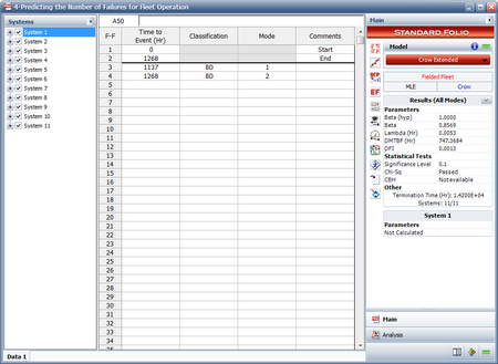
- 1) The next figure shows the estimated Crow Extended parameters.
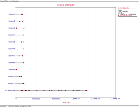
- 2) Upon observing the estimated parameter [math]\displaystyle{ \beta \,\! }[/math], it does appear that the systems were randomly ordered since [math]\displaystyle{ \beta =0.8569\,\! }[/math]. This value is close to 1. You can also verify that the confidence bounds on [math]\displaystyle{ \beta \,\! }[/math] include 1 by going to the QCP and calculating the parameter bounds or by viewing the Beta Bounds plot. However, you can also determine graphically if the systems were randomly ordered by using the System Operation plot as shown below. Looking at the Cum. Time Line, it does not appear that the failures have a trend associated with them. Therefore, the systems can be assumed to be randomly ordered.


