General Log-Linear Relationship

This article also appears in the Accelerated Life Testing Data Analysis Reference book.

When a test involves multiple accelerating stresses or requires the inclusion of an engineering variable, a general multivariable relationship is needed. Such a relationship is the general log-linear relationship, which describes a life characteristic as a function of a vector of [math]\displaystyle{ n\,\! }[/math] stresses, or [math]\displaystyle{ \underline{X}=({{X}_{1}},{{X}_{2}}...{{X}_{n}}).\,\! }[/math] ALTA includes this relationship and allows up to eight stresses. Mathematically the relationship is given by:

[math]\displaystyle{ L(\underline{X})={{e}^{{{\alpha }_{0}}+\underset{j=1}{\overset{n}{\mathop{\sum }}}\,{{\alpha }_{j}}{{X}_{j}}}}\,\! }[/math]

where:

• [math]\displaystyle{ {{\alpha }_{0}}\,\! }[/math] and [math]\displaystyle{ {{\alpha }_{j}}\,\! }[/math] are model parameters.

• [math]\displaystyle{ X\,\! }[/math] is a vector of [math]\displaystyle{ n\,\! }[/math] stresses.

This relationship can be further modified through the use of transformations and can be reduced to the relationships discussed previously, if so desired. As an example, consider a single stress application of this relationship and an inverse transformation on [math]\displaystyle{ X,\,\! }[/math] such that [math]\displaystyle{ V=1/X\,\! }[/math] or:

[math]\displaystyle{ \begin{align} & L(V)= & {{e}^{{{\alpha }_{0}}+\tfrac{{{\alpha }_{1}}}{V}}} =\ & {{e}^{{{\alpha }_{0}}}}{{e}^{\tfrac{{{\alpha }_{1}}}{V}}} \end{align}\,\! }[/math]

It can be easily seen that the generalized log-linear relationship with a single stress and an inverse transformation has been reduced to the Arrhenius relationship, where:

[math]\displaystyle{ \begin{align} & C= & {{e}^{{{\alpha }_{0}}}} \\ & B= & {{\alpha }_{1}} \end{align}\,\! }[/math]

or:

[math]\displaystyle{ L(V)=C{{e}^{\tfrac{B}{V}}}\,\! }[/math]

Similarly, when one chooses to apply a logarithmic transformation on [math]\displaystyle{ X\,\! }[/math] such that [math]\displaystyle{ V=\ln (X)\,\! }[/math], the relationship would reduce to the Inverse Power Law relationship. Furthermore, if more than one stress is present, one could choose to apply a different transformation to each stress to create combination relationships similar to the Temperature-Humidity and the Temperature-Non Thermal. ALTA has three built-in transformation options, namely:

None	X=V	Exponential LSR
Reciprocal	[math]\displaystyle{ V=1/X\,\! }[/math]	Arrhenius LSR
Logarithmic	[math]\displaystyle{ V=\ln (X)\,\! }[/math]	Power LSR

The power of the relationship and this formulation becomes evident once one realizes that 6,651 unique life-stress relationships are possible (when allowing a maximum of eight stresses). When combined with the life distributions available in ALTA, almost 20,000 models can be created.

Using the GLL Model

Like the previous relationships, the general log-linear relationship can be combined with any of the available life distributions by expressing a life characteristic from that distribution with the GLL relationship. A brief overview of the GLL-distribution models available in ALTA is presented next.

GLL Exponential

The GLL-exponential model can be derived by setting [math]\displaystyle{ m=L(\underline{X})\,\! }[/math] in the exponential pdf, yielding the following GLL-exponential pdf:

[math]\displaystyle{ f(t,\underline{X})={{e}^{-\left( {{\alpha }_{0}}+\underset{j=1}{\overset{n}{\mathop{\sum }}}\,{{\alpha }_{j}}{{X}_{j}} \right)}}{{e}^{-\left( {{\alpha }_{0}}+\underset{j=1}{\overset{n}{\mathop{\sum }}}\,{{\alpha }_{j}}{{X}_{j}} \right)\cdot t}}\,\! }[/math]

The total number of unknowns to solve for in this model is [math]\displaystyle{ n+1\,\! }[/math] (i.e., [math]\displaystyle{ {{a}_{0}},{{a}_{1}},...{{a}_{n}}).\,\! }[/math]

GLL Weibull

The GLL-Weibull model can be derived by setting [math]\displaystyle{ \eta =L(\underline{X})\,\! }[/math] in Weibull pdf, yielding the following GLL-Weibull pdf:

[math]\displaystyle{ f(t,\underline{X})=\beta \cdot {{t}^{\beta -1}}{{e}^{-\beta \left( {{\alpha }_{0}}+\underset{j=1}{\overset{n}{\mathop{\sum }}}\,{{\alpha }_{j}}{{X}_{j}} \right)}}{{e}^{-{{t}^{\beta }}{{e}^{-\beta \left( {{\alpha }_{0}}+\underset{j=1}{\overset{n}{\mathop{\sum }}}\,{{\alpha }_{j}}{{X}_{j}} \right)}}}}\,\! }[/math]

The total number of unknowns to solve for in this model is [math]\displaystyle{ n+2\,\! }[/math] (i.e., [math]\displaystyle{ \beta ,{{a}_{0}},{{a}_{1}},...{{a}_{n}}).\,\! }[/math]

GLL Lognormal

The GLL-lognormal model can be derived by setting [math]\displaystyle{ \breve{T}=L(\underline{X})\,\! }[/math] in the lognormal pdf, yielding the following GLL-lognormal pdf:

[math]\displaystyle{ f(t,\underline{X})=\frac{1}{t\text{ }{{\sigma }_{{{T}'}}}\sqrt{2\pi }}{{e}^{-\tfrac{1}{2}{{\left( \tfrac{{T}'-{{\alpha }_{0}}-\underset{j=1}{\overset{n}{\mathop{\sum }}}\,{{\alpha }_{j}}{{X}_{j}}}{{{\sigma }_{{{T}'}}}} \right)}^{2}}}}\,\! }[/math]

The total number of unknowns to solve for in this model is [math]\displaystyle{ n+2\,\! }[/math] (i.e., [math]\displaystyle{ {{\sigma }_{{{T}'}}},{{a}_{0}},{{a}_{1}},...{{a}_{n}}).\,\! }[/math]

GLL Likelihood Function

The maximum likelihood estimation method can be used to determine the parameters for the GLL relationship and the selected life distribution. For each distribution, the likelihood function can be derived, and the parameters of model (the distribution parameters and the GLL parameters) can be obtained by maximizing the log-likelihood function. For example, the log-likelihood function for the Weibull distribution is given by:

[math]\displaystyle{ \begin{align} & \ln (L)= & \Lambda =\underset{i=1}{\overset{{{F}_{e}}}{\mathop \sum }}\,{{N}_{i}}\ln \left[ \beta \cdot T_{i}^{\beta -1}{{e}^{-T_{i}^{\beta }\cdot {{e}^{-\beta \left( {{\alpha }_{0}}+\mathop{\sum}_{j=1}^{n}{{a}_{j}}{{x}_{i,j}} \right)}}}}{{e}^{-\beta \left( {{\alpha }_{0}}+\mathop{\sum}_{j=1}^{n}{{a}_{j}}{{x}_{i,j}} \right)}} \right] -\underset{i=1}{\overset{S}{\mathop \sum }}\,N_{i}^{\prime }{{\left( T_{i}^{\prime } \right)}^{\beta }}{{e}^{-\beta \left( {{\alpha }_{0}}+\mathop{\sum}_{j=1}^{n}{{a}_{j}}{{x}_{i,j}} \right)}}+\overset{FI}{\mathop{\underset{i=1}{\mathop{\underset{}{\overset{}{\mathop \sum }}\,}}\,}}\,N_{i}^{\prime \prime }\ln [R_{Li}^{\prime \prime }-R_{Ri}^{\prime \prime }] \end{align}\,\! }[/math]

where:

[math]\displaystyle{ \begin{align} & R_{Li}^{\prime \prime }= & {{e}^{-{{\left( T_{Li}^{\prime \prime }{{e}^{{{\alpha }_{0}}+\underset{j=1}{\mathop{\overset{n}{\mathop{\mathop{}_{}^{}}}\,}}\,{{\alpha }_{j}}{{x}_{j}}}} \right)}^{\beta }}}} \\ & R_{Ri}^{\prime \prime }= & {{e}^{-{{\left( T_{Ri}^{\prime \prime }{{e}^{{{\alpha }_{0}}+\underset{j=1}{\mathop{\overset{n}{\mathop{\mathop{}_{}^{}}}\,}}\,{{\alpha }_{j}}{{x}_{j}}}} \right)}^{\beta }}}} \end{align}\,\! }[/math]

and:

• [math]\displaystyle{ {{F}_{e}}\,\! }[/math] is the number of groups of exact times-to-failure data points.

• [math]\displaystyle{ {{N}_{i}}\,\! }[/math] is the number of times-to-failure in the [math]\displaystyle{ {{i}^{th}}\,\! }[/math] time-to-failure data group.

• [math]\displaystyle{ \lambda \,\! }[/math] is the failure rate parameter (unknown).

• [math]\displaystyle{ {{T}_{i}}\,\! }[/math] is the exact failure time of the [math]\displaystyle{ {{i}^{th}}\,\! }[/math] group.

• [math]\displaystyle{ S\,\! }[/math] is the number of groups of suspension data points.

• [math]\displaystyle{ N_{i}^{\prime }\,\! }[/math] is the number of suspensions in the [math]\displaystyle{ {{i}^{th}}\,\! }[/math] group of suspension data points.

• [math]\displaystyle{ T_{i}^{\prime }\,\! }[/math] is the running time of the [math]\displaystyle{ {{i}^{th}}\,\! }[/math] suspension data group.

• [math]\displaystyle{ FI\,\! }[/math] is the number of interval data groups.

• [math]\displaystyle{ N_{i}^{\prime \prime }\,\! }[/math] is the number of intervals in the [math]\displaystyle{ {{i}^{th}}\,\! }[/math] group of data intervals.

• [math]\displaystyle{ T_{Li}^{\prime \prime }\,\! }[/math] is the beginning of the [math]\displaystyle{ {{i}^{th}}\,\! }[/math] interval.

• [math]\displaystyle{ T_{Ri}^{\prime \prime }\,\! }[/math] is the ending of the [math]\displaystyle{ {{i}^{th}}\,\! }[/math] interval.

GLL Example

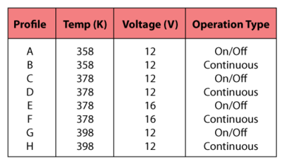
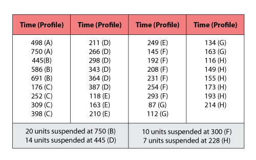
Consider the data summarized in the following tables. These data illustrate a typical three-stress type accelerated test.

Stress Profile Summary

Failure Data

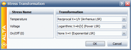
The data in the second table are analyzed assuming a Weibull distribution, an Arrhenius life-stress relationship for temperature and an inverse power life-stress relationship for voltage. No transformation is performed on the operation type. The operation type variable is treated as an indicator variable that takes a discrete value of 0 for an on/off operation and 1 for a continuous operation. The following figure shows the stress types and their transformations in ALTA.

The GLL relationship then becomes:

[math]\displaystyle{ \eta ={{e}^{{{\alpha }_{0}}+{{\alpha }_{1}}\tfrac{1}{{{V}_{1}}}+{{\alpha }_{2}}\ln ({{V}_{2}})+{{\alpha }_{3}}{{V}_{3}}}}\,\! }[/math]

The resulting relationship after performing these transformations is:

[math]\displaystyle{ \begin{align} & \eta = & {{e}^{{{\alpha }_{0}}}}{{e}^{{{\alpha }_{1}}\tfrac{1}{{{V}_{1}}}}}{{e}^{{{\alpha }_{2}}\ln ({{V}_{2}})}}{{e}^{{{\alpha }_{3}}{{V}_{3}}}} =\ & {{e}^{{{\alpha }_{0}}}}{{e}^{{{\alpha }_{1}}\tfrac{1}{{{V}_{1}}}}}V_{2}^{{{\alpha }_{2}}}{{e}^{{{\alpha }_{3}}{{V}_{3}}}} \end{align}\,\! }[/math]

Therefore, the parameter [math]\displaystyle{ B\,\! }[/math] of the Arrhenius relationship is equal to the log-linear coefficient [math]\displaystyle{ {{\alpha }_{1}}\,\! }[/math], and the parameter [math]\displaystyle{ n\,\! }[/math] of the inverse power relationship is equal to ([math]\displaystyle{ -{{\alpha}_{2}}\,\! }[/math]). Therefore [math]\displaystyle{ \eta \,\! }[/math] can also be written as:

[math]\displaystyle{ \eta ={{e}^{{{\alpha }_{0}}}}{{e}^{\tfrac{B}{{{V}_{1}}}}}V_{2}^{n}{{e}^{{{\alpha }_{3}}{{V}_{3}}}}\,\! }[/math]

The activation energy of the Arrhenius relationship can be calculated by multiplying B with Boltzmann's constant.

The best fit values for the parameters in this case are:

[math]\displaystyle{ \begin{align} \beta = & 3.7483;\text{ }{{\alpha }_{0}} = -6.0220;\text{ }{{\alpha }_{1}} = 5776.9341; \\ {{\alpha }_{2}} = & -1.4340;\text{ }{{\alpha }_{3}} = 0.6242. \end{align}\,\! }[/math]

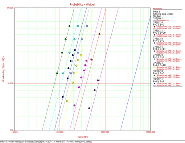
Once the parameters are estimated, further analysis on the data can be performed. First, using ALTA, a Weibull probability plot of the data can be obtained, as shown next.

Several types of information about the model as well as the data can be obtained from a probability plot. For example, the choice of an underlying distribution and the assumption of a common slope (shape parameter) can be examined. In this example, the linearity of the data supports the use of the Weibull distribution. In addition, the data appear parallel on this plot, therefore reinforcing the assumption of a common beta. Further statistical analysis can and should be performed for these purposes as well.

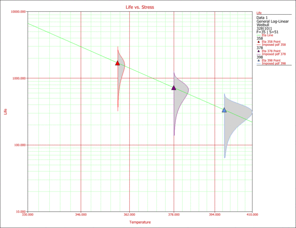
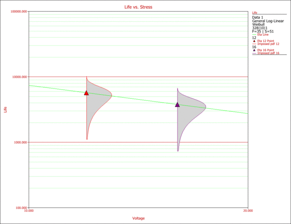
The Life vs. Stress plot is a very common plot for the analysis of accelerated data. Life vs. Stress plots can be very useful in assessing the effect of each stress on a product's failure. In this case, since the life is a function of three stresses, three different plots can be created. Such plots are created by holding two of the stresses constant at the desired use level, and varying the remaining one. The use stress levels for this example are 328K for temperature and 10V for voltage. For the operation type, a decision has to be made by the engineers as to whether they implement an on/off or continuous operation. The next two figures display the effects of temperature and voltage on the life of the product.

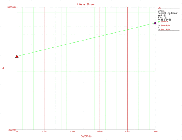
The effects of the two different operation types on life can be observed in the next figure. It can be seen that the on/off cycling has a greater effect on the life of the product in terms of accelerating failure than the continuous operation. In other words, a higher reliability can be achieved by running the product continuously.

Indicator Variables

Another advantage of the multivariable relationships included in ALTA is that they allow for simultaneous analysis of continuous and categorical variables. Categorical variables are variables that take on discrete values such as the lot designation for products from different manufacturing lots. In this example, lot is a categorical variable, and it can be expressed in terms of indicator variables. Indicator variables only take a value of 1 or 0. For example, consider a sample of test units. A number of these units were obtained from Lot 1, others from Lot 2, and the rest from Lot 3. These three lots can be represented with the use of indicator variables, as follows:

• Define two indicator variables, [math]\displaystyle{ {{X}_{1}}\,\! }[/math] and [math]\displaystyle{ {{X}_{2}}.\,\! }[/math]

• For the units from Lot 1, [math]\displaystyle{ {{X}_{1}}=1,\,\! }[/math] and [math]\displaystyle{ {{X}_{2}}=0.\,\! }[/math]

• For the units from Lot 2, [math]\displaystyle{ {{X}_{1}}=0,\,\! }[/math] and [math]\displaystyle{ {{X}_{2}}=1.\,\! }[/math]

• For the units from Lot 3, [math]\displaystyle{ {{X}_{1}}=0,\,\! }[/math] and [math]\displaystyle{ {{X}_{2}}=0.\,\! }[/math]

Assume that an accelerated test was performed with these units, and temperature was the accelerated stress. In this case, the GLL relationship can be used to analyze the data. From this relationship we get:

[math]\displaystyle{ L(\underline{X})={{e}^{{{\alpha }_{0}}+{{\alpha }_{1}}{{X}_{1}}+{{\alpha }_{2}}{{X}_{2}}+{{\alpha }_{3}}{{X}_{3}}}}\,\! }[/math]

where:

• [math]\displaystyle{ {{X}_{1}}\,\! }[/math] and [math]\displaystyle{ {{X}_{2}}\,\! }[/math] are the indicator variables, as defined above.

• [math]\displaystyle{ {{X}_{3}}=\tfrac{1}{T},\,\! }[/math] where [math]\displaystyle{ T\,\! }[/math] is the temperature.

The data can now be entered in ALTA and, with the assumption of an underlying life distribution and using MLE, the parameters of this model can be obtained.