Additional Information on Load Sharing

As presented in earlier chapters, a reliability block diagram (RBD) allows you to graphically represent how the components within a system are reliability-wise connected. In most cases, independence is assumed across the components within the system. For example, the failure of component A does not affect the failure of component B. However, if a system consists of components that are sharing a load, then the assumption of independence no longer holds true.

If one component fails, then the component(s) that are still operating will have to assume the failed unit's portion of the load. Therefore, the reliabilities of the surviving unit(s) will change. Calculating the system reliability is no longer an easy proposition. In the case of load sharing components, the change of the failure distributions of the surviving components must be known in order to determine the system's reliability.

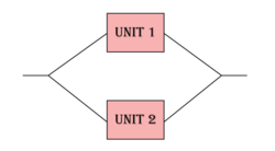
To illustrate this, consider a system of two units connected reliability-wise in parallel as shown below.

Assume that the units must supply an output of 8 volts and that if both units are operational, each unit is to supply 50% of the total output. If one of the units fails, then the surviving unit supplies 100%. Furthermore, assume that having to supply the entire load has a negative impact on the reliability characteristics of the surviving unit. Because the reliability characteristics of the unit change based on whether both or only one is operating, a life distribution along with a life-stress relationship (as discussed in A Brief Introduction to Life-Stress Relationships) will be needed to model each component.

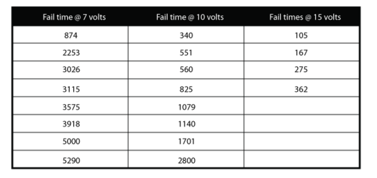
To illustrate the steps needed, we will create the model starting from raw data. Assume that a total of 20 units were tested to failure at 7, 10 and 15 volts. The test data set is presented in the next table.

For this example, Units 1 and 2 are the same component. Therefore, only one set of data was collected. However, it is possible that the load sharing components in a system may not be the same. If that were the case, data would need to be collected for each component.

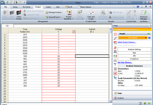
The data set was analyzed using ReliaSoft's ALTA software (as shown in the figure below) with the Inverse Power Law as the underlying life-stress relationship and Weibull as the life distribution.

The estimated model parameters, [math]\displaystyle{ \beta \,\! }[/math], [math]\displaystyle{ K\,\! }[/math] and [math]\displaystyle{ n\,\! }[/math], are shown next.

[math]\displaystyle{ \begin{align} \beta = & 1.9239 \\ K= & 3.2387\times {{10}^{-7}} \\ n= & 3.4226 \end{align}\,\! }[/math]

Or:

[math]\displaystyle{ \begin{align} {{R}_{1}}(t,{{S}_{1}})= & {{e}^{-{{\left( KS_{1}^{n}t \right)}^{\beta }}}} \\ = & {{e}^{-{{\left( 3.2387\times {{10}^{-7}}S_{1}^{3.4226}t \right)}^{1.9239}}}} \ \end{align}\,\! }[/math].

[math]\displaystyle{ {{f}_{1}}(t,{{S}_{1}})=\beta KS_{1}^{n}{{\left( KS_{1}^{n}t \right)}^{\beta -1}}{{e}^{-{{\left( KS_{1}^{n}t \right)}^{\beta }}}} \ \,\! }[/math]

And for this case:

[math]\displaystyle{ \begin{align} {{R}_{1}}(t,{{S}_{1}})= & {{R}_{2}}(t,{{S}_{2}}) \\ {{f}_{1}}(t,{{S}_{1}})= & {{f}_{2}}(t,{{S}_{2}}) \end{align}\,\! }[/math]

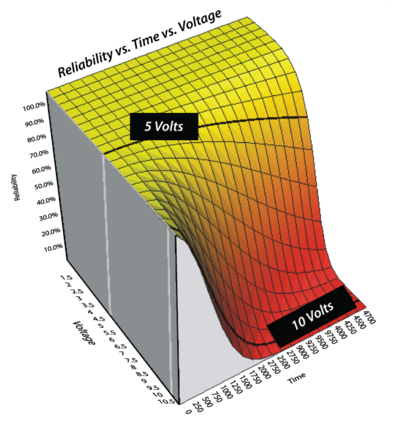
The figure below shows a plot of [math]\displaystyle{ {{R}_{1}}(t,{{S}_{1}})={{e}^{-{{\left( KS_{1}^{n}t \right)}^{\beta }}}} = {{e}^{-{{\left( 3.2387\times {{10}^{-7}}S_{1}^{3.4226}t \right)}^{1.9239}}}}\ \,\! }[/math].

Now that the failure properties have been determined using the test data, the reliability of the system at some time, [math]\displaystyle{ t\,\! }[/math], can be calculated using the following equation:

[math]\displaystyle{ \begin{align} R(t,S)= & {{R}_{1}}(t,{{S}_{1}})\cdot {{R}_{2}}(t,{{S}_{2}}) \\ & +\underset{o}{\overset{t}{\mathop \int }}\,{{f}_{1}}\left( x,{{S}_{1}} \right)\cdot {{R}_{2}}(x,{{S}_{2}})\cdot \left( \frac{{{R}_{2}}({{t}_{1e}}+(t-x),S)}{{{R}_{2}}({{t}_{1e}},S)} \right)dx \\ & +\underset{o}{\overset{t}{\mathop \int }}\,{{f}_{2}}\left( x,{{S}_{2}} \right)\cdot {{R}_{1}}(x,{{S}_{1}})\cdot \left( \frac{{{R}_{1}}({{t}_{2e}}+(t-x),S)}{{{R}_{1}}({{t}_{2e}},S)} \right)dx \end{align}\,\! }[/math]

where:

[math]\displaystyle{ \begin{align} {{S}_{1}}= & {{P}_{1}}S \\ {{S}_{2}}= & {{P}_{2}}S \end{align}\,\! }[/math]

And:

• [math]\displaystyle{ S\,\! }[/math] is the total load (or required output).

• [math]\displaystyle{ {{P}_{1}}\,\! }[/math] and [math]\displaystyle{ {{P}_{2}}\,\! }[/math] are the portion of the total load that each unit supports when both units are operational. In this case, [math]\displaystyle{ {{P}_{1}}={{P}_{2}}=0.5=50%.\,\! }[/math]

• [math]\displaystyle{ {{S}_{1}}\,\! }[/math] and [math]\displaystyle{ {{S}_{2}}\,\! }[/math] represent the portions of the load that Unit 1 and Unit 2 must support when both units are operational.

• [math]\displaystyle{ {{t}_{{{1}_{e}}}}\,\! }[/math] is the equivalent operating time for Unit 1 if it had been operating at [math]\displaystyle{ S\,\! }[/math] instead of [math]\displaystyle{ {{S}_{1}}\,\! }[/math]. A graphical representation of the equivalent time is shown in the following figure, where the curve marked by L represents the low stress (load) and the curve marked by H represents the high stress (load).

[math]\displaystyle{ {{t}_{1e}}\,\! }[/math] can be calculated by:

[math]\displaystyle{ \begin{align} {{R}_{1}}(t)= & {{R}_{1}}({{t}_{1e}}) \\ {{e}^{-{{(tKS_{1}^{n})}^{\beta }}}}= & {{e}^{-{{({{t}_{1e}}K{{S}^{n}})}^{\beta }}}} \\ tS_{1}^{n}= & {{t}_{1e}}{{S}^{n}} \\ {{t}_{1e}}= & t{{\left( \frac{{{S}_{1}}}{S} \right)}^{n}},\text{ }{{S}_{1}}={{P}_{1}}S \\ \therefore & {{t}_{1e}}=tP_{1}^{n} \end{align}\,\! }[/math]

[math]\displaystyle{ {{t}_{2e}}\,\! }[/math] can be calculated the same way, or:

[math]\displaystyle{ \begin{align} {{R}_{2}}(t)= & {{R}_{2}}({{t}_{2e}}) \\ \therefore & {{t}_{2e}}=tP_{2}^{n} \end{align}\,\! }[/math]

In this example, the reliability equations for Unit 1 and Unit 2 are the same since they are the same type of component and demonstrate the same failure properties. In addition, the total output is divided equally between the two units (when both units are operating), so [math]\displaystyle{ {{t}_{1e}}\,\! }[/math] and [math]\displaystyle{ {{t}_{2e}}\,\! }[/math] will also be the same.

The next step is to determine the reliability of the system after 8,760 hours, [math]\displaystyle{ R(t=8,760)\,\! }[/math]. Using

[math]\displaystyle{ \begin{align} R(t,S)= & {{R}_{1}}(t,{{S}_{1}})\cdot {{R}_{2}}(t,{{S}_{2}}) \\ & +\underset{o}{\overset{t}{\mathop \int }}\,{{f}_{1}}\left( x,{{S}_{1}} \right)\cdot {{R}_{2}}(x,{{S}_{2}})\cdot \left( \frac{{{R}_{2}}({{t}_{1e}}+(t-x),S)}{{{R}_{2}}({{t}_{1e}},S)} \right)dx \\ & +\underset{o}{\overset{t}{\mathop \int }}\,{{f}_{2}}\left( x,{{S}_{2}} \right)\cdot {{R}_{1}}(x,{{S}_{1}})\cdot \left( \frac{{{R}_{1}}({{t}_{2e}}+(t-x),S)}{{{R}_{1}}({{t}_{2e}},S)} \right)dx \end{align}\,\! }[/math]

the system reliability is found to be:

[math]\displaystyle{ \begin{align} R(t=8760)= & 0.8567 \\ = & 85.67% \end{align}\,\! }[/math]

Load Sharing in BlockSim

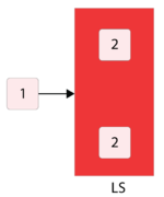
BlockSim uses this formulation when computing reliabilities of units in a load sharing configuration. When using the System Reliability Equation window, BlockSim returns a single token for the reliability of units in a load sharing configuration (as well as in the case of standby redundancy, discussed in the next section). As an example, consider the following RBD with Unit 1 in series with a container that includes two load sharing units.

BlockSim will return the system equation as:

[math]\displaystyle{ {{R}_{System}}=+{{R}_{LS}}\cdot {{R}_{1}}\,\! }[/math]

where [math]\displaystyle{ {{R}_{LS}}\,\! }[/math] implies a form similar to:

[math]\displaystyle{ \begin{align} R(t,S)= & {{R}_{1}}(t,{{S}_{1}})\cdot {{R}_{2}}(t,{{S}_{2}}) \\ & +\underset{o}{\overset{t}{\mathop \int }}\,{{f}_{1}}\left( x,{{S}_{1}} \right)\cdot {{R}_{2}}(x,{{S}_{2}})\cdot \left( \frac{{{R}_{2}}({{t}_{1e}}+(t-x),S)}{{{R}_{2}}({{t}_{1e}},S)} \right)dx \\ & +\underset{o}{\overset{t}{\mathop \int }}\,{{f}_{2}}\left( x,{{S}_{2}} \right)\cdot {{R}_{1}}(x,{{S}_{1}})\cdot \left( \frac{{{R}_{1}}({{t}_{2e}}+(t-x),S)}{{{R}_{1}}({{t}_{2e}},S)} \right)dx \end{align}\,\! }[/math]

BlockSim allows for k-out-of-n units in a load sharing configuration.

Example

A component has five possible failure modes, [math]\displaystyle{ A\,\! }[/math], [math]\displaystyle{ {{B}_{A}}\,\! }[/math], [math]\displaystyle{ {{B}_{B}}\,\! }[/math], [math]\displaystyle{ {{B}_{C}}\,\! }[/math] and [math]\displaystyle{ C\,\! }[/math]. The [math]\displaystyle{ B\,\! }[/math] modes are interdependent. In addition:

• The system will fail if mode [math]\displaystyle{ A\,\! }[/math] occurs, mode [math]\displaystyle{ C\,\! }[/math] occurs or two out of the three [math]\displaystyle{ B\,\! }[/math] modes occur.

• Modes [math]\displaystyle{ A\,\! }[/math] and [math]\displaystyle{ C\,\! }[/math] each have a Weibull distribution, with a [math]\displaystyle{ \beta =2\,\! }[/math] and [math]\displaystyle{ \eta =10,000\,\! }[/math] and [math]\displaystyle{ 15,000\,\! }[/math] hours, respectively.

• Events [math]\displaystyle{ {{B}_{A}}\,\! }[/math], [math]\displaystyle{ {{B}_{B}}\,\! }[/math] and [math]\displaystyle{ {{B}_{C}}\,\! }[/math] each have an exponential distribution with a mean of 10,000 hours.

• If any [math]\displaystyle{ B\,\! }[/math] event occurs (i.e., [math]\displaystyle{ {{B}_{A}}\,\! }[/math], [math]\displaystyle{ {{B}_{B}}\,\! }[/math] or [math]\displaystyle{ {{B}_{C}}\,\! }[/math] ), the remaining [math]\displaystyle{ B\,\! }[/math] events are more likely to occur. Specifically, the mean times of the remaining [math]\displaystyle{ B\,\! }[/math] events are halved.

Determine the reliability at 1,000 hours for this component.

Solution

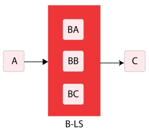
The first step is to create the RBD. Modes [math]\displaystyle{ A\,\! }[/math], [math]\displaystyle{ C\,\! }[/math] and a load sharing container with the [math]\displaystyle{ {{B}_{i}}\,\! }[/math] modes must be drawn in series, as illustrated next.

The next step is to define the properties for each block, including those for the container. Based on the problem statement, the [math]\displaystyle{ B\,\! }[/math] modes are in a 2-out-of-3 load sharing redundancy. When all three are working (i.e., when no [math]\displaystyle{ B\,\! }[/math] mode has occurred), each block has an exponential distribution with [math]\displaystyle{ \mu=10,000\,\! }[/math].

The next step is to set the weight proportionality factor. This factor defines the portion of the load that the particular item carries while operating, as well as the load that shifts to the remaining units upon failure of the item. To illustrate, assume three units (A, B and C) are in a load sharing container with weight proportionality factors of 1, 2 and 3 respectively (and a 1-out-of-3 requirement).

• Unit A carries [math]\displaystyle{ \left( \tfrac{1}{1+2+3} \right)=0.166\,\! }[/math] or 16.6% of the total load.

• Unit B carries [math]\displaystyle{ \left( \tfrac{2}{1+2+3} \right)=0.333\,\! }[/math] or 33.3% of the total load.

• Unit C carries [math]\displaystyle{ \left( \tfrac{3}{1+2+3} \right)=0.50\,\! }[/math] or 50% of the total load.

The actual load on each unit then becomes the product of the entire load defined for the container times the portion carried by that unit. For example, if the container load is 100 lbs, then the portion assigned to Unit A will be [math]\displaystyle{ 100\cdot 0.166=16.6\,\! }[/math] lbs.

In the current example, all [math]\displaystyle{ B\,\! }[/math] modes share the same load and thus, have equal weight proportionality factors. Because these factors are relative, if the same number is used for all three [math]\displaystyle{ B\,\! }[/math] modes then the results will be the same. Thus, the weight proportionality factor is set equal to 1 for each [math]\displaystyle{ B\,\! }[/math] mode.

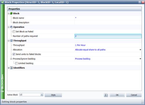
The last properties that need to be defined are the total load and the 2-out-of-3 redundancy. The total load is dependent on how the parameters were computed. In this case, the total load was assumed to be 3 when the parameters were computed (i.e., the load per item was 1 when all worked and 1.5 when two worked). For the 2-out-of-3 redundancy, the following figure shows the Block Properties window of the load sharing container with the number of paths set to 2. When all of the parameters have been specified in BlockSim, the reliability at 1,000 hours can be determined. From the Analytical QCP, this is found to be 98.1048%.