Exponential Distribution Examples
New format available! This reference is now available in a new format that offers faster page load, improved display for calculations and images and more targeted search.
As of January 2024, this Reliawiki page will not continue to be updated. Please update all links and bookmarks to the latest references at Weibull examples and Weibull reference examples.
These examples also appear in the Life Data Analysis Reference book.
Exponential Distribution for Grouped Data
20 units were reliability tested with the following results:
| Table - Life Test Data | |
| Number of Units in Group | Time-to-Failure |
|---|---|
| 7 | 100 |
| 5 | 200 |
| 3 | 300 |
| 2 | 400 |
| 1 | 500 |
| 2 | 600 |
1. Assuming a 2-parameter exponential distribution, estimate the parameters by hand using the MLE analysis method.
2. Repeat the above using Weibull++. (Enter the data as grouped data to duplicate the results.)
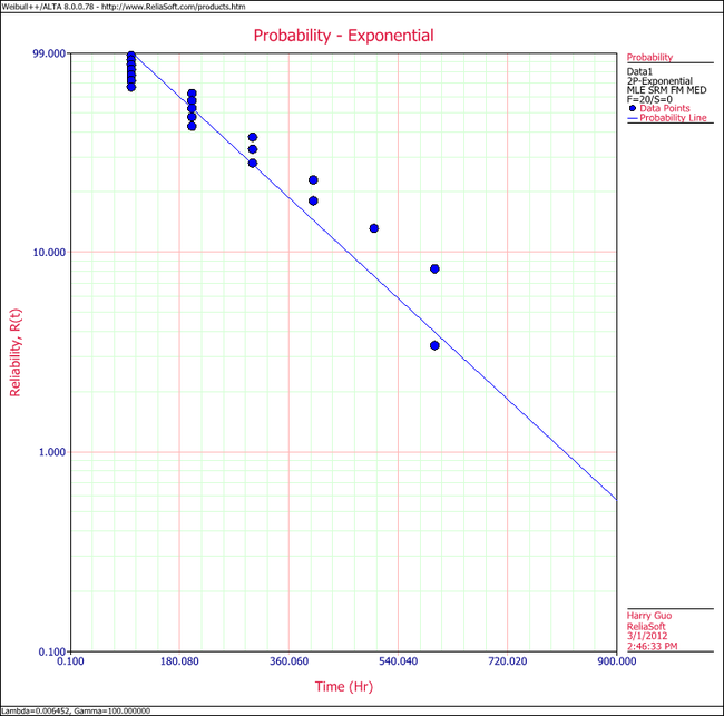
3. Show the Probability plot for the analysis results.
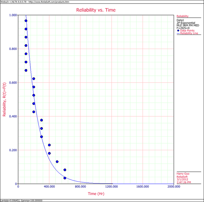
4. Show the Reliability vs. Time plot for the results.
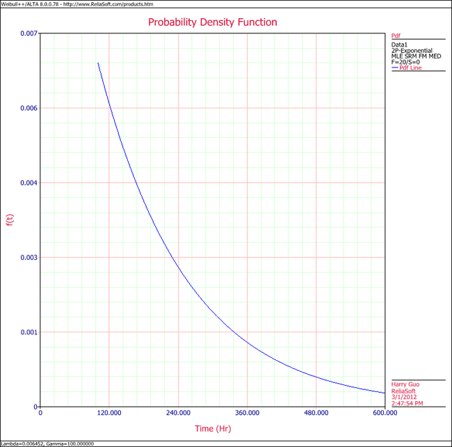
5. Show the pdf plot for the results.
6. Show the Failure Rate vs. Time plot for the results.
7. Estimate the parameters using the rank regression on Y (RRY) analysis method (and using grouped ranks).
Solution
1. For the 2-parameter exponential distribution and for [math]\displaystyle{ \hat{\gamma }=100\,\! }[/math] hours (first failure), the partial of the log-likelihood function, [math]\displaystyle{ \lambda\,\! }[/math], becomes:
- [math]\displaystyle{ \begin{align} \frac{\partial \Lambda }{\partial \lambda }= &\underset{i=1}{\overset{6}{\mathop \sum }}\,{N_i} \left[ \frac{1}{\lambda }-\left( {{T}_{i}}-100 \right) \right]=0\\ \Rightarrow & 7[\frac{1}{\lambda }-(100-100)]+5[\frac{1}{\lambda}-(200-100)] + \ldots +2[\frac{1}{\lambda}-(600-100)]\\ = & 0\\ \Rightarrow & \hat{\lambda}=\frac{20}{3100}=0.0065 \text{fr/hr} \end{align} \,\! }[/math]
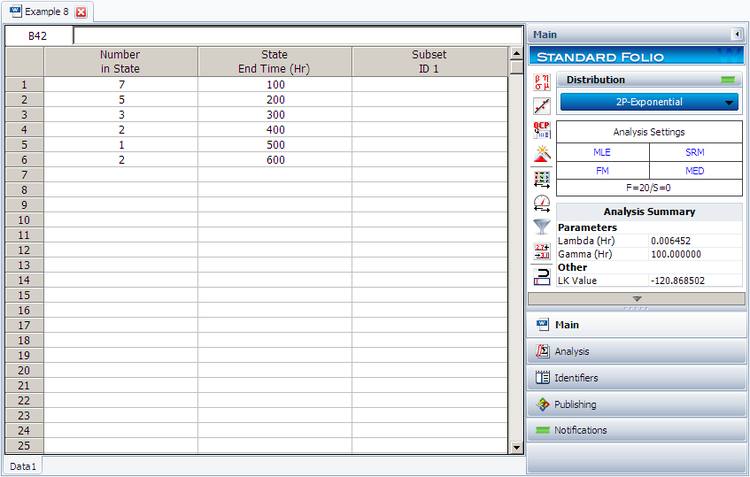
2. Enter the data in a Weibull++ standard folio and calculate it as shown next.
3. On the Plot page of the folio, the exponential Probability plot will appear as shown next.
4. View the Reliability vs. Time plot.
5. View the pdf plot.
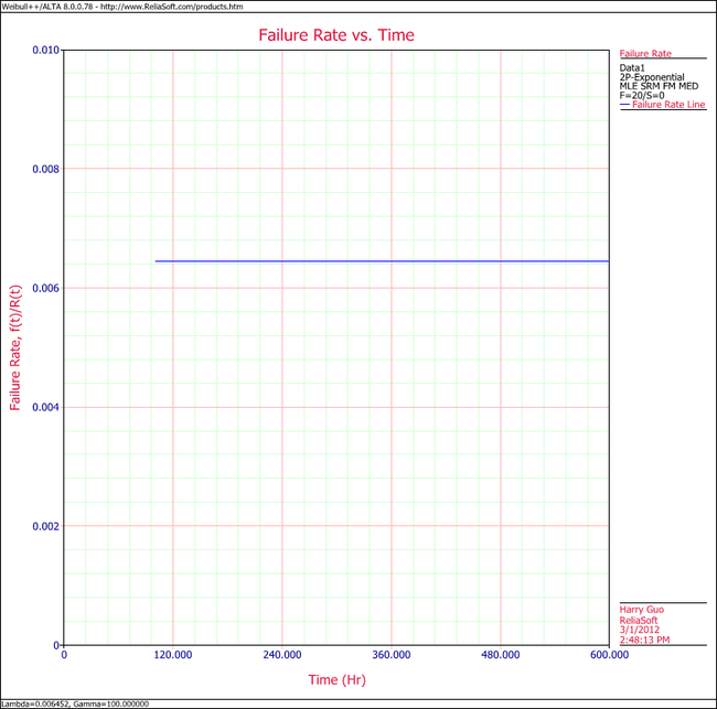
6. View the Failure Rate vs. Time plot.
Note that, as described at the beginning of this chapter, the failure rate for the exponential distribution is constant. Also note that the Failure Rate vs. Time plot does show values for times before the location parameter, [math]\displaystyle{ \gamma \,\! }[/math], at 100 hours.
7. In the case of grouped data, one must be cautious when estimating the parameters using a rank regression method. This is because the median rank values are determined from the total number of failures observed by time [math]\displaystyle{ {{T}_{i}}\,\! }[/math] where [math]\displaystyle{ i\,\! }[/math] indicates the group number. In this example, the total number of groups is [math]\displaystyle{ N=6\,\! }[/math] and the total number of units is [math]\displaystyle{ {{N}_{T}}=20\,\! }[/math]. Thus, the median rank values will be estimated for 20 units and for the total failed units ([math]\displaystyle{ {{N}_{{{F}_{i}}}}\,\! }[/math]) up to the [math]\displaystyle{ {{i}^{th}}\,\! }[/math] group, for the [math]\displaystyle{ {{i}^{th}}\,\! }[/math] rank value. The median ranks values can be found from rank tables or they can be estimated using ReliaSoft's Quick Statistical Reference tool.
For example, the median rank value of the fourth group will be the [math]\displaystyle{ {{17}^{th}}\,\! }[/math] rank out of a sample size of twenty units (or 81.945%).
The following table is then constructed.
Given the values in the table above, calculate [math]\displaystyle{ \hat{a}\,\! }[/math] and [math]\displaystyle{ \hat{b}\,\! }[/math]:
- [math]\displaystyle{ \begin{align} & \hat{b}= & \frac{\underset{i=1}{\overset{6}{\mathop{\sum }}}\,{{t}_{i}}{{y}_{i}}-(\underset{i=1}{\overset{6}{\mathop{\sum }}}\,{{t}_{i}})(\underset{i=1}{\overset{6}{\mathop{\sum }}}\,{{y}_{i}})/6}{\underset{i=1}{\overset{6}{\mathop{\sum }}}\,t_{i}^{2}-{{(\underset{i=1}{\overset{6}{\mathop{\sum }}}\,{{t}_{i}})}^{2}}/6} \\ & & \\ & \hat{b}= & \frac{-4320.3362-(2100)(-9.6476)/6}{910,000-{{(2100)}^{2}}/6} \end{align}\,\! }[/math]
or:
- [math]\displaystyle{ \hat{b}=-0.005392\,\! }[/math]
and:
- [math]\displaystyle{ \hat{a}=\overline{y}-\hat{b}\overline{t}=\frac{\underset{i=1}{\overset{N}{\mathop{\sum }}}\,{{y}_{i}}}{N}-\hat{b}\frac{\underset{i=1}{\overset{N}{\mathop{\sum }}}\,{{t}_{i}}}{N}\,\! }[/math]
or:
- [math]\displaystyle{ \hat{a}=\frac{-9.6476}{6}-(-0.005392)\frac{2100}{6}=0.2793\,\! }[/math]
Therefore:
- [math]\displaystyle{ \hat{\lambda }=-\hat{b}=-(-0.005392)=0.05392\text{ failures/hour}\,\! }[/math]
and:
- [math]\displaystyle{ \hat{\gamma }=\frac{\hat{a}}{\hat{\lambda }}=\frac{0.2793}{0.005392}\,\! }[/math]
or:
- [math]\displaystyle{ \hat{\gamma }\simeq 51.8\text{ hours}\,\! }[/math]
Then:
- [math]\displaystyle{ f(T)=(0.005392){{e}^{-0.005392(T-51.8)}}\,\! }[/math]
Using Weibull++, the estimated parameters are:
- [math]\displaystyle{ \begin{align} \hat{\lambda }= & 0.0054\text{ failures/hour} \\ \hat{\gamma }= & 51.82\text{ hours} \end{align}\,\! }[/math]
The small difference in the values from Weibull++ is due to rounding. In the application, the calculations and the rank values are carried out up to the [math]\displaystyle{ 15^{th}\,\! }[/math] decimal point.
Exponential Distribution with Auto Batch Run
A number of leukemia patients were treated with either drug 6MP or a placebo, and the times in weeks until cancer symptoms returned were recorded. Analyze each treatment separately [21, p.175].
| Table - Leukemia Treatment Results | |||
| Time (weeks) | Number of Patients | Treament | Comments |
|---|---|---|---|
| 1 | 2 | placebo | |
| 2 | 2 | placebo | |
| 3 | 1 | placebo | |
| 4 | 2 | placebo | |
| 5 | 2 | placebo | |
| 6 | 4 | 6MP | 3 patients completed |
| 7 | 1 | 6MP | |
| 8 | 4 | placebo | |
| 9 | 1 | 6MP | Not completed |
| 10 | 2 | 6MP | 1 patient completed |
| 11 | 2 | placebo | |
| 11 | 1 | 6MP | Not completed |
| 12 | 2 | placebo | |
| 13 | 1 | 6MP | |
| 15 | 1 | placebo | |
| 16 | 1 | 6MP | |
| 17 | 1 | placebo | |
| 17 | 1 | 6MP | Not completed |
| 19 | 1 | 6MP | Not completed |
| 20 | 1 | 6MP | Not completed |
| 22 | 1 | placebo | |
| 22 | 1 | 6MP | |
| 23 | 1 | placebo | |
| 23 | 1 | 6MP | |
| 25 | 1 | 6MP | Not completed |
| 32 | 2 | 6MP | Not completed |
| 34 | 1 | 6MP | Not completed |
| 35 | 1 | 6MP | Not completed |
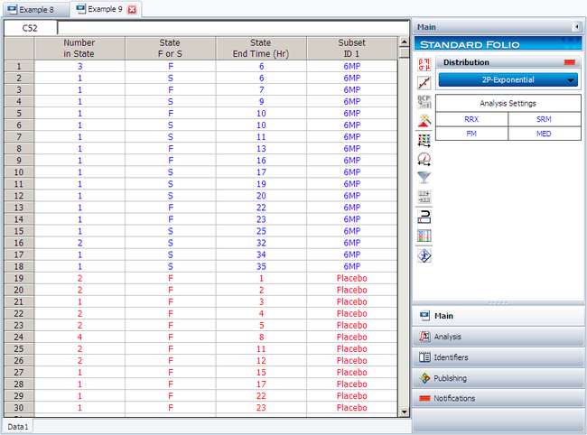
Create a new Weibull++ standard folio that's configured for grouped times-to-failure data with suspensions. In the first column, enter the number of patients. Whenever there are uncompleted tests, enter the number of patients who completed the test separately from the number of patients who did not (e.g., if 4 patients had symptoms return after 6 weeks and only 3 of them completed the test, then enter 1 in one row and 3 in another). In the second column enter F if the patients completed the test and S if they didn't. In the third column enter the time, and in the fourth column (Subset ID) specify whether the 6MP drug or a placebo was used.
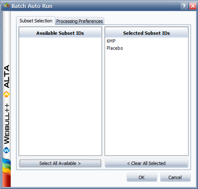
Next, open the Batch Auto Run utility and select to separate the 6MP drug from the placebo, as shown next.
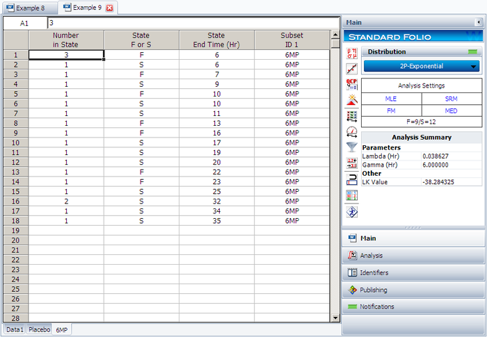
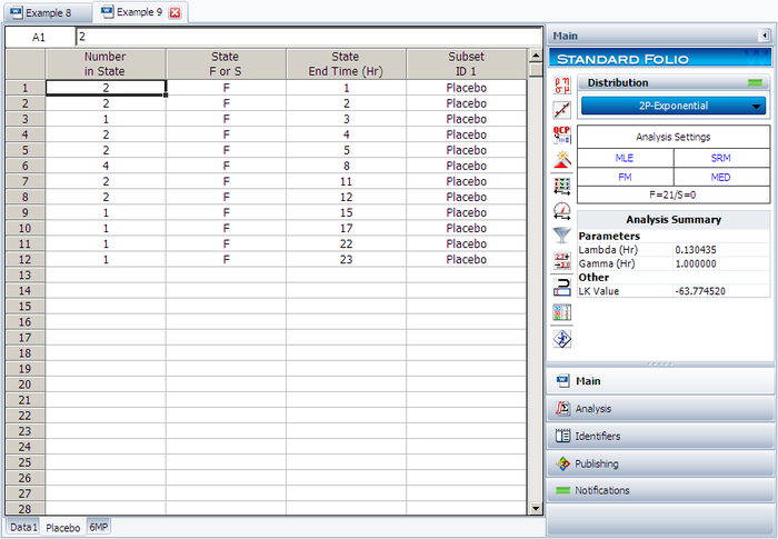
The software will create two data sheets, one for each subset ID, as shown next.
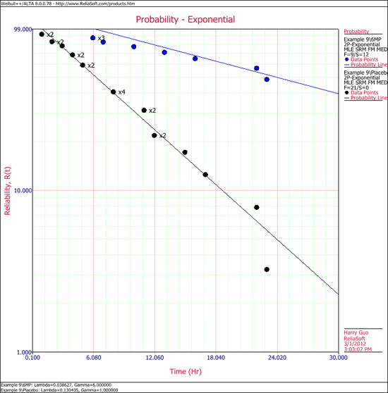
Calculate both data sheets using the 2-parameter exponential distribution and the MLE analysis method, then insert an additional plot and select to show the analysis results for both data sheets on that plot, which will appear as shown next.

