Template:Parameter estimation logistic rga
Parameter Estimation
Example 1
Using the reliability growth data given in Table 8.1, do the following:
- 1) Find a Gompertz curve that represents the data and plot it with the raw data.
- 2) Find a Logistic reliability growth curve that represents the data and plot it with the raw data.
| Time, months | Raw Data Reliability (%) | Gompertz Reliability (%) | Logistic Reliablity (%) |
|---|---|---|---|
| 0 | 31.00 | 24.85 | 22.73 |
| 1 | 35.50 | 38.48 | 38.14 |
| 2 | 49.30 | 51.95 | 56.37 |
| 3 | 70.10 | 63.82 | 73.02 |
| 4 | 83.00 | 73.49 | 85.01 |
| 5 | 92.20 | 80.95 | 92.24 |
| 6 | 96.40 | 86.51 | 96.14 |
| 7 | 98.60 | 90.54 | 98.12 |
| 8 | 99.00 | 93.41 | 99.09 |
Solution
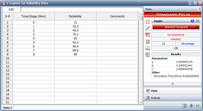
- 1) Figure Logistic1 shows the entered data and the estimated parameters using the Standard Gompertz model.
- Therefore:
- [math]\displaystyle{ \begin{align} & \widehat{a}= & 0.9999 \\ & \widehat{b}= & 0.2485 \\ & \widehat{c}= & 0.6858 \end{align} }[/math]
- [math]\displaystyle{ R=(0.9999){{(0.2485)}^{{{0.6858}^{T}}}} }[/math]
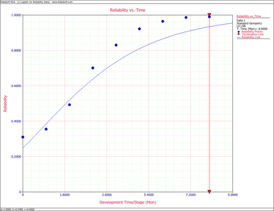
The values of predicted reliabilities are plotted in Figure Logig81.
Notice how the Standard Gompertz model is not really capable of handling the S-shaped characteristics of this data.
- 2. The least squares estimators of the Logistic growth curve parameters are [9]:
- where:
- [math]\displaystyle{ \begin{align} & {{{\hat{b}}}_{1}}= & \frac{\underset{i=0}{\overset{N-1}{\mathop{\sum }}}\,{{T}_{i}}{{Y}_{i}}-N\cdot \bar{T}\cdot \bar{Y}}{\underset{i=0}{\overset{N-1}{\mathop{\sum }}}\,T_{i}^{2}-N\cdot {{{\bar{T}}}^{2}}} \\ & {{{\hat{b}}}_{0}}= & \bar{Y}-{{{\hat{b}}}_{1}}\bar{T} \\ & {{Y}_{i}}= & \ln \left( \frac{1}{{{R}_{i}}}-1 \right) \\ & \bar{Y}= & \frac{1}{N}\underset{i=0}{\overset{N-1}{\mathop \sum }}\,{{Y}_{i}} \end{align} }[/math]
In this example [math]\displaystyle{ N=9 }[/math] , which gives:
From Eqns. (eq37) and (eq38):
And from Eqns. (eq36a) and (eq36b):
- [math]\displaystyle{ \begin{align} & \widehat{b}= & {{e}^{1.2235}} \\ & = & 3.3991 \\ & \widehat{k}= & -(-0.7398) \\ & = & 0.7398 \end{align} }[/math]
Therefore, the Logistic reliability growth curve that represents this data set is given by:
- [math]\displaystyle{ R=\frac{1}{1+3.3991\,{{e}^{-0.7398\,T}}} }[/math]
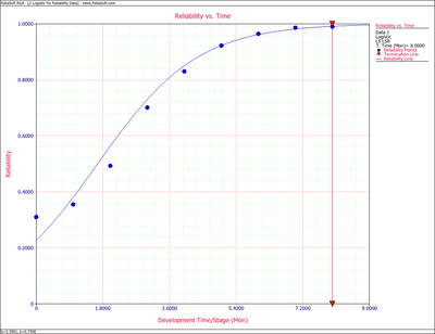
Figure Logig82 shows the Reliability vs. Time plot. The plot shows that the observed data set is estimated well by the Logistic reliability growth curve, except in the region closely surrounding the inflection point of the observed reliability. This problem can be overcome by using the Modified Gompertz model, which was presented in Chapter 7.
Example 2
A prototype was tested under a success/failure pattern. The test consisted of 15 runs and Table 8.2 presents the data from the test. Find the Logistic model that best fits the data set and plot it along with the reliability observed from the raw data.
| Time | Result | Observed Reliability |
|---|---|---|
| 0 | F | 0.5000 |
| 1 | F | 0.3333 |
| 2 | S | 0.5000 |
| 3 | S | 0.6000 |
| 4 | F | 0.5000 |
| 5 | S | 0.5714 |
| 6 | S | 0.6250 |
| 7 | S | 0.6667 |
| 8 | S | 0.7000 |
| 9 | F | 0.6364 |
| 10 | S | 0.6667 |
| 11 | S | 0.6923 |
| 12 | S | 0.7143 |
| 13 | S | 0.7333 |
Solution
The first run is ignored because it was a success and the reliability at that point was 100%. This failure will be ignored throughout the analysis because it is considered that the test starts when the reliability is not equal to zero or one. The test essentially begins at time 1, and is now considered as time 0 with [math]\displaystyle{ N=14 }[/math] . The observed reliability is shown in the last column of Table 8.2. Keep in mind that the observed reliability values still account for the initial suspension.
Eqn. (eq41a) becomes:
- [math]\displaystyle{ \begin{align} & \bar{Y}= & \frac{1}{N}\underset{i=0}{\overset{N-1}{\mathop \sum }}\,{{Y}_{i}} \\ & = & \frac{1}{14}\underset{i=0}{\overset{13}{\mathop \sum }}\,\ln \left( \frac{1}{{{R}_{i}}}-1 \right) \\ & = & -0.43163 \end{align} }[/math]
- and:
- [math]\displaystyle{ \begin{align} & \bar{T}= & \frac{1}{14}\underset{i=0}{\overset{13}{\mathop \sum }}\,{{T}_{i}} \\ & = & 6.5 \\ & \underset{i=0}{\overset{13}{\mathop \sum }}\,T_{i}^{2}= & 819.0 \\ & \underset{i=0}{\overset{13}{\mathop \sum }}\,{{T}_{i}}{{Y}_{i}}= & -61.69 \end{align} }[/math]
Now, from the least squares estimators, Eqns. (eq37) and (eq38) are:
- Therefore:
- [math]\displaystyle{ \begin{align} & \widehat{b}= & {{e}^{0.2087}} \\ & = & 1.2321 \\ & \widehat{k}= & -(-0.0985) \\ & = & 0.0985 \end{align} }[/math]
The Logistic reliability model that best fits the data is given by:
- [math]\displaystyle{ R=\frac{1}{1+1.2321\cdot \ \,{{e}^{-0.0985T}}} }[/math]
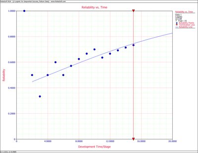
Figure Logig83 shows the Reliability vs. Time plot.
Example 3
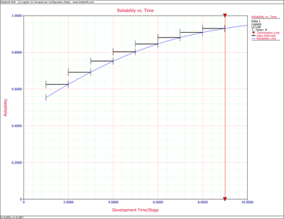
Some equipment underwent testing in different stages. The testing may have been performed in subsequent days, weeks or months with an unequal number of units tested every day. Each group was tested and several failures occurred. The data set is given in columns 1 and 2 of Table 8.3. Find the Logistic model that best fits the data and plot it along with the reliability observed from the raw data.
| Number of Units | Number of Failures | [math]\displaystyle{ T_i }[/math] | Observed Reliability |
|---|---|---|---|
| 10 | 5 | 0 | 0.5000 |
| 8 | 3 | 1 | 0.6250 |
| 9 | 3 | 2 | 0.6667 |
| 9 | 2 | 3 | 0.7778 |
| 10 | 2 | 4 | 0.8000 |
| 10 | 1 | 5 | 0.9000 |
| 10 | 1 | 6 | 0.9000 |
| 10 | 1 | 7 | 0.9000 |
| 10 | 1 | 8 | 0.9000 |
Solution
The observed reliability is [math]\displaystyle{ 1-\tfrac{\#\text{ of failures}}{\#\text{ of units}} }[/math] and the last column of Table 8.3 shows the values for each group. With [math]\displaystyle{ N=9 }[/math] , Eqn. (eq41a) becomes:
- [math]\displaystyle{ \begin{align} & \bar{Y}= & \frac{1}{9}\underset{i=0}{\overset{8}{\mathop \sum }}\,\ln \left( \frac{1}{{{R}_{i}}}-1 \right) \\ & = & -1.4036 \end{align} }[/math]
- and:
- [math]\displaystyle{ \begin{align} & \bar{T}= & \frac{1}{9}\underset{i=0}{\overset{8}{\mathop \sum }}\,{{T}_{i}} \\ & = & 4 \\ & \underset{i=0}{\overset{8}{\mathop \sum }}\,T_{i}^{2}= & 204 \\ & \underset{i=0}{\overset{8}{\mathop \sum }}\,{{T}_{i}}{{Y}_{i}}= & -68.33 \end{align} }[/math]
Now from the least squares estimators, Eqns. (eq37) and (eq38) give:
- [math]\displaystyle{ \begin{align} & {{{\hat{b}}}_{1}}= & \frac{\underset{i=0}{\overset{8}{\mathop{\sum }}}\,{{T}_{i}}{{Y}_{i}}-N\cdot \bar{T}\cdot \bar{Y}}{\underset{i=0}{\overset{8}{\mathop{\sum }}}\,T_{i}^{2}-N\cdot {{{\bar{T}}}^{2}}} \\ & = & \frac{-68.33-9\cdot 4\cdot \left( -1.4036 \right)}{204-9\cdot {{4}^{2}}} \\ & = & -0.2967 \\ & & \\ & {{{\hat{b}}}_{0}}= & \bar{Y}-{{{\hat{b}}}_{1}}\bar{T} \\ & = & \left( -1.4036 \right)-\left( -0.2967 \right)\cdot 4.0 \\ & = & -0.2168 \end{align} }[/math]
- Therefore:
- [math]\displaystyle{ \begin{align} & \widehat{b}= & {{e}^{-0.2168}} \\ & = & 0.8051 \\ & \widehat{k}= & -(-0.2967) \\ & = & 0.2967 \end{align} }[/math]
The Logistic reliability model that best fits the data is given by:
- [math]\displaystyle{ R=\frac{1}{1+0.8051\cdot \ \,{{e}^{-0.2967T}}} }[/math]
Figure Logig85 shows the Reliability vs. Time plot.
