Template:Mixed data rga
Mixed Data
The Crow Extended model also can be applied for discrete data from one-shot (success/failure) testing. In RGA, the Discrete Data > Mixed Data option gives a data sheet that can accommodate data from tests where a single unit is tested for each successive configuration (individual trial-by-trial), where multiple units are tested for each successive configuration (configurations in groups) or a combination of both. This data sheet can be analyzed with either the Crow-AMSAA (NHPP) model or the Crow Extended model. Corrective actions cannot take place at the time of failure for discrete data. With that in mind, the mixed data type does not allow for BC modes. For discrete data there are only A or BD modes. In terms of practical applications, think of a growth test for missile systems. Since these are one-shot items, the fixes to failure modes are delayed until at least the next trial. Note that for calculation purposes it is required to have at least three failures in the first interval. If that is not the case, then the data set needs to be grouped before calculating. RGA performs this operation in the background.
Example 5
A one-shot system underwent reliability growth testing for a total of 20 trials. The test was performed as a combination of groups of units with the same configuration and individual trials. Table 9.5 shows the obtained data set. The "Failures in Interval" column specifies the number of failures that occurred in each interval and the "Cumulative Trials" column specifies the cumulative number of trials at the end of that interval. In other words, the first three rows contain the data from the first trial, in which 8 units with the same configuration were tested and 3 failures (with different failure modes) were observed. The next row contains data from the second trial, in which 2 units with the same configuration were tested and no failures occurred. And so on.
| Table 9.5 - Mixed data for Example 5 | |||
| Failures in Interval | Cumulative Trials | Classification | Mode |
|---|---|---|---|
| 1 | 8 | BD | 1 |
| 1 | 8 | BD | 2 |
| 1 | 8 | BD | 3 |
| 0 | 10 | ||
| 0 | 11 | ||
| 0 | 12 | ||
| 1 | 13 | BD | 2 |
| 0 | 14 | ||
| 0 | 15 | ||
| 1 | 16 | BD | 4 |
| 0 | 17 | ||
| 0 | 18 | ||
| 0 | 18 | ||
| 1 | 20 | BD | 5 |
The table also gives the classifications of the failure modes. There are 5 BD modes. The average effectiveness factor for the BD modes is [math]\displaystyle{ 0.7 }[/math] . Do the following:
- 1) Calculate the demonstrated reliability at the end of the test.
- 2) Calculate the growth potential reliability.
Solution
Based on the equations presented in Chapter 5, the parameters of the Crow-AMSAA (NHPP) model are estimated as follows:
- [math]\displaystyle{ \widehat{\beta }=0.8572 }[/math]
- and:
- [math]\displaystyle{ \widehat{\lambda }=0.4602 }[/math]
However, since there are only A or BD modes for mixed data, there is no growth during the test. In other words, the hypothesis for the [math]\displaystyle{ \widehat{\beta } }[/math] parameter is that [math]\displaystyle{ \widehat{\beta }=1. }[/math]
From Chapter 5, we know that:
- [math]\displaystyle{ \widehat{\lambda }=\frac{n}{T_{n}^{\widehat{\beta }}} }[/math]
or, if [math]\displaystyle{ \widehat{\beta }=1 }[/math] , this becomes:
- [math]\displaystyle{ \begin{align} & \widehat{\lambda }= & \frac{n}{{{T}_{n}}} \\ & = & \frac{6}{20} \\ & = & 0.3 \end{align} }[/math]
As we have seen, the Crow-AMSAA instantaneous failure intensity, [math]\displaystyle{ {{\lambda }_{i}}(T) }[/math] , is defined as:
- [math]\displaystyle{ {{\lambda }_{i}}(T)=\lambda \beta {{T}^{\beta -1}},\text{with }T\gt 0,\text{ }\lambda \gt 0\text{ and }\beta \gt 0 }[/math]
Using trials instead of time, and accommodating for [math]\displaystyle{ \widehat{\beta }=1 }[/math] , we can calculate the instantaneous failure probability at the end of the test, or [math]\displaystyle{ T=20 }[/math] :
- [math]\displaystyle{ {{Q}_{i}}(20)=\widehat{\lambda }=0.3 }[/math]
So the instantaneous reliability at the end of the test, or demonstrated reliability, is:
- [math]\displaystyle{ \begin{align} & {{R}_{i}}(20)= & 1-{{Q}_{i}}(20) \\ & = & 1-0.3 \\ & = & 0.7 \end{align} }[/math]
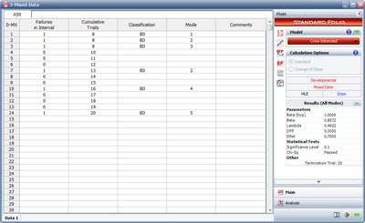
Figure mixed Crow Extended folio shows the data sheet of Table 9.5 as calculated in RGA.
Based on Eqn. (extendedGP), the growth potential unreliability is:
- [math]\displaystyle{ \begin{align} & {{\widehat{Q}}_{GP}}(T)= & \left( \frac{{{N}_{A}}}{T}+\underset{i=1}{\overset{M}{\mathop \sum }}\,(1-{{d}_{i}})\frac{{{N}_{i}}}{T} \right) \\ & = & \underset{i=1}{\overset{M}{\mathop \sum }}\,(1-0.7)\frac{{{N}_{i}}}{T} \\ & = & 0.3*(\frac{1+1+1+1+1+1)}{20} \\ & = & 0.09 \end{align} }[/math]
So the growth potential reliability is:
- [math]\displaystyle{ \begin{align} & {{\widehat{R}}_{GP}}(T)= & 1-{{\widehat{Q}}_{GP}}(T) \\ & = & 1-0.09 \\ & = & 0.91 \end{align} }[/math]
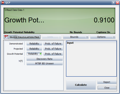
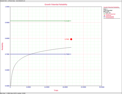
Figure mixedrowxtendedCP shows the calculation of the growth potential reliability for the mixed data using the QCP in RGA. Figure MixedrowxtendedPlot shows the growth potential plot for this example.


