Template:Data analysis fleet rsa
Data Analysis
Once the accumulated timeline has been generated, it is then converted into grouped data. To accomplish this, a group interval is required. The group interval length should be chosen so that it is representative of the data. Also note that the intervals do not have to be of equal length. Once the data points have been grouped, the parameters can be obtained using maximum likelihood estimation as described in Chapter 5 in the Grouped Data Analysis section. The data in Table 13.2 can be grouped into 5 hr intervals. This interval length is sufficiently large to insure that there are failures within each interval. The grouped data set is given in Table 13.3.
| Table 13.3 - Grouped data | |
| Failures in Interval | Interval End Time |
|---|---|
| 1 | 5 |
| 1 | 10 |
| 1 | 15 |
| 1 | 20 |
| 1 | 25 |
The Crow-AMSAA model for Grouped Failure Times is used for the data in Table 13.3 and the parameters of the model are solved by satisfying the following maximum likelihood equations (Chapter 5).
- [math]\displaystyle{ \begin{matrix} \widehat{\lambda }=\frac{n}{T_{k}^{\widehat{\beta }}} \\ \underset{i=1}{\overset{k}{\mathop \sum }}\,{{n}_{i}}\left[ \frac{T_{i}^{\widehat{\beta }}\ln {{T}_{i-1}}-T_{i-1}^{\widehat{\beta }}\ln {{T}_{i-1}}}{T_{i}^{\widehat{\beta }}-T_{i-1}^{\widehat{\beta }}}-\ln {{T}_{k}} \right]=0 \\ \end{matrix} }[/math]
Example 4
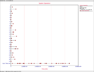
Table 13.4 presents data for a fleet of 27 systems. A cycle is a complete history from overhaul to overhaul. The failure history for the last completed cycle for each system is recorded. This is a random sample of data from the fleet. These systems are in the order in which they were selected. Suppose the intervals to group the current data are 10000, 20000, 30000, 40000 and the final interval is defined by the termination time. Conduct the fleet analysis.
| Table 13.4 - Sample fleet data | |||
| System | Cycle Time [math]\displaystyle{ {{T}_{j}} }[/math] | Number of failures [math]\displaystyle{ {{N}_{j}} }[/math] | Failure Time [math]\displaystyle{ {{X}_{ij}} }[/math] |
|---|---|---|---|
| 1 | 1396 | 1 | 1396 |
| 2 | 4497 | 1 | 4497 |
| 3 | 525 | 1 | 525 |
| 4 | 1232 | 1 | 1232 |
| 5 | 227 | 1 | 227 |
| 6 | 135 | 1 | 135 |
| 7 | 19 | 1 | 19 |
| 8 | 812 | 1 | 812 |
| 9 | 2024 | 1 | 2024 |
| 10 | 943 | 2 | 316, 943 |
| 11 | 60 | 1 | 60 |
| 12 | 4234 | 2 | 4233, 4234 |
| 13 | 2527 | 2 | 1877, 2527 |
| 14 | 2105 | 2 | 2074, 2105 |
| 15 | 5079 | 1 | 5079 |
| 16 | 577 | 2 | 546, 577 |
| 17 | 4085 | 2 | 453, 4085 |
| 18 | 1023 | 1 | 1023 |
| 19 | 161 | 1 | 161 |
| 20 | 4767 | 2 | 36, 4767 |
| 21 | 6228 | 3 | 3795, 4375, 6228 |
| 22 | 68 | 1 | 68 |
| 23 | 1830 | 1 | 1830 |
| 24 | 1241 | 1 | 1241 |
| 25 | 2573 | 2 | 871, 2573 |
| 26 | 3556 | 1 | 3556 |
| 27 | 186 | 1 | 186 |
| Total | 52110 | 37 | |
Solution
For the system data in Table 13.4, the data can be grouped into 10000, 20000, 30000, 4000 and 52110 time intervals. Table 13.5 gives the grouped data.
| Table 13.5 - Grouped data | |
| Time | Observed Failures |
|---|---|
| 10000 | 8 |
| 20000 | 16 |
| 30000 | 22 |
| 40000 | 27 |
| 52110 | 37 |
Based on the above time intervals, the maximum likelihood estimates of [math]\displaystyle{ \widehat{\lambda } }[/math] and [math]\displaystyle{ \widehat{\beta } }[/math] for this data set are then given by:
- [math]\displaystyle{ \begin{matrix} \widehat{\lambda }=0.00147 \\ \widehat{\beta }=0.93328 \\ \end{matrix} }[/math]
Figure fle shows the System Operation plot.
[math]\displaystyle{ }[/math]
