Expected Failure Times Plot Example

New format available! This reference is now available in a new format that offers faster page load, improved display for calculations and images and more targeted search.

As of January 2024, this Reliawiki page will not continue to be updated. Please update all links and bookmarks to the latest references at Weibull examples and Weibull reference examples.

---

This example appears in the Life Data Analysis Reference book.

Example: Using the Expected Failure Times Plot for Test Design

4 units were allocated for a reliability test. The test engineers want to know how long the test will last if all the units are tested to failure. Based on previous experiments, they assume the underlying failure distribution is a Weibull distribution with [math]\displaystyle{ \beta }[/math] = 2 and [math]\displaystyle{ \eta }[/math] = 500.

Solution

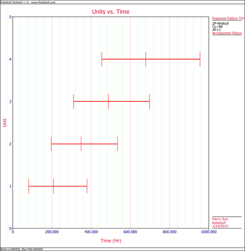
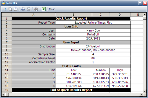
Using Weibull++'s Expected Failure Times plot, the expected failure times with 80% 2-sided confidence bounds are given below.

From the above results, we can see the upper bound of the last failure is about 955 hours. Therefore, the test probably will last for around 955 hours.

As we know, with 4 samples, the median rank for the second failure is 0.385728. Using this value and the assumed Weibull distribution, the median value of the failure time of the second failure is calculated as:

[math]\displaystyle{ \begin{align} & Q=1-{{e}^-{{{\left( \frac{t}{\eta } \right)}^{\beta }}}}\Rightarrow \\ & \ln (1-Q)={{\left( \frac{t}{\eta } \right)}^{\beta }} \\ & \Rightarrow t=\text{349.04}\\ \end{align} }[/math]

Its bounds and other failure times can be calculated in a similar way.