Time-Dependent System Reliability for Components in Parallel

New format available! This reference is now available in a new format that offers faster page load, improved display for calculations and images and more targeted search.

As of January 2024, this Reliawiki page will not continue to be updated. Please update all links and bookmarks to the latest references at BlockSim examples and BlockSim reference examples.

---

This example appears in the System Analysis Reference book.

Time-Dependent System Reliability for Components with Constant Failure Rates in Parallel

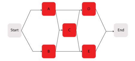
Consider the system shown next.

Components [math]\displaystyle{ A\,\! }[/math] through [math]\displaystyle{ E\,\! }[/math] are Weibull distributed with [math]\displaystyle{ \beta =1.2\,\! }[/math] and [math]\displaystyle{ \eta =1230\,\! }[/math] hours. The starting and ending blocks cannot fail.

Determine the following:

• The reliability equation for the system and its corresponding plot.

• The system's pdf and its corresponding plot.

• The system's failure rate equation and the corresponding plot.

• The MTTF.

• The warranty time for a 90% reliability.

• The reliability for a 200-hour mission, if it is known that the system has already successfully operated for 200 hours.

Solution

The first step is to obtain the reliability function for the system. The methods described in the previous chapter can be employed, such as the event space or path-tracing methods. Using BlockSim, the following reliability equation is obtained:

[math]\displaystyle{ \begin{align} {{R}_{s}}(t)= & ({{R}_{Start}}\cdot {{R}_{End}}(2{{R}_{A}}\cdot {{R}_{D}}\cdot {{R}_{C}}\cdot {{R}_{B}}\cdot {{R}_{E}} \\ & -{{R}_{A}}\cdot {{R}_{D}}\cdot {{R}_{C}}\cdot {{R}_{B}}-{{R}_{A}}\cdot {{R}_{D}}\cdot {{R}_{C}}\cdot {{R}_{E}} \\ & -{{R}_{A}}\cdot {{R}_{D}}\cdot {{R}_{B}}\cdot {{R}_{E}}-{{R}_{A}}\cdot {{R}_{C}}\cdot {{R}_{B}}\cdot {{R}_{E}} \\ & -{{R}_{D}}\cdot {{R}_{C}}\cdot {{R}_{B}}\cdot {{R}_{E}}+{{R}_{A}}\cdot {{R}_{C}}\cdot {{R}_{E}} \\ & +{{R}_{D}}\cdot {{R}_{C}}\cdot {{R}_{B}}+{{R}_{A}}\cdot {{R}_{D}}+{{R}_{B}}\cdot {{R}_{E}})) \end{align} }[/math]

Note that since the starting and ending blocks cannot fail, [math]\displaystyle{ {{R}_{Start}}=1\,\! }[/math] and [math]\displaystyle{ {{R}_{End}}=1,\,\! }[/math] equation above can be reduced to:

[math]\displaystyle{ \begin{align} {{R}_{s}}(t)= & 2\cdot {{R}_{A}}\cdot {{R}_{D}}\cdot {{R}_{C}}\cdot {{R}_{B}}\cdot {{R}_{E}} \\ & -{{R}_{A}}\cdot {{R}_{D}}\cdot {{R}_{C}}\cdot {{R}_{B}}-{{R}_{A}}\cdot {{R}_{D}}\cdot {{R}_{C}}\cdot {{R}_{E}} \\ & -{{R}_{A}}\cdot {{R}_{D}}\cdot {{R}_{B}}\cdot {{R}_{E}}-{{R}_{A}}\cdot {{R}_{C}}\cdot {{R}_{B}}\cdot {{R}_{E}} \\ & -{{R}_{D}}\cdot {{R}_{C}}\cdot {{R}_{B}}\cdot {{R}_{E}}+{{R}_{A}}\cdot {{R}_{C}}\cdot {{R}_{E}} \\ & +{{R}_{D}}\cdot {{R}_{C}}\cdot {{R}_{B}}+{{R}_{A}}\cdot {{R}_{D}}+{{R}_{B}}\cdot {{R}_{E}} \end{align} }[/math]

where [math]\displaystyle{ {{R}_{A}}\,\! }[/math] is the reliability equation for Component A, or:

[math]\displaystyle{ {{R}_{A}}(t)={{e}^{-{{\left( \tfrac{t}{{{\eta }_{A}}} \right)}^{{{\beta }_{A}}}}}} }[/math]

[math]\displaystyle{ {{R}_{B}}\,\! }[/math] is the reliability equation for Component [math]\displaystyle{ B\,\! }[/math] , etc.

Since the components in this example are identical, the system reliability equation can be further reduced to:

[math]\displaystyle{ \begin{align} {{R}_{s}}(t)=2R{{(t)}^{2}}+2R{{(t)}^{3}}-5R{{(t)}^{4}}+2R{{(t)}^{5}} \end{align} }[/math]

Or, in terms of the failure distribution:

[math]\displaystyle{ {{R}_{s}}(t)=2\cdot {{e}^{-2{{\left( \tfrac{t}{\eta } \right)}^{\beta }}}}+2\cdot {{e}^{-3{{\left( \tfrac{t}{\eta } \right)}^{\beta }}}}-5\cdot {{e}^{-4{{\left( \tfrac{t}{\eta } \right)}^{\beta }}}}+2\cdot {{e}^{-5{{\left( \tfrac{t}{\eta } \right)}^{\beta }}}} }[/math]

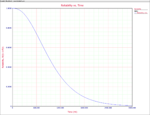
The corresponding plot is given in the following figure.

In order to obtain the system's pdf, the derivative of the reliability equation given above is taken with respect to time, resulting in:

[math]\displaystyle{ \begin{align} {{f}_{s}}(t)= & 4\cdot \frac{\beta }{\eta }{{\left( \frac{t}{\eta } \right)}^{\beta -1}}{{e}^{-2{{\left( \tfrac{t}{\eta } \right)}^{\beta }}}}+6\cdot \frac{\beta }{\eta }{{\left( \frac{t}{\eta } \right)}^{\beta -1}}{{e}^{-3{{\left( \tfrac{t}{\eta } \right)}^{\beta }}}} \\ & -20\cdot \frac{\beta }{\eta }{{\left( \frac{t}{\eta } \right)}^{\beta -1}}{{e}^{-4{{\left( \tfrac{t}{\eta } \right)}^{\beta }}}}+10\cdot \frac{\beta }{\eta }{{\left( \frac{t}{\eta } \right)}^{\beta -1}}{{e}^{-5{{\left( \tfrac{t}{\eta } \right)}^{\beta }}}} \end{align} }[/math]

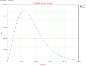
The pdf can now be plotted for different time values, [math]\displaystyle{ t\,\! }[/math] , as shown in the following figure.

The system's failure rate can now be obtained by dividing the system's pdf given in equation above by the system's reliability function given in [math]\displaystyle{ {{R}_{s}}(t)=2\cdot {{e}^{-2{{\left( \tfrac{t}{\eta } \right)}^{\beta }}}}+2\cdot {{e}^{-3{{\left( \tfrac{t}{\eta } \right)}^{\beta }}}}-5\cdot {{e}^{-4{{\left( \tfrac{t}{\eta } \right)}^{\beta }}}}+2\cdot {{e}^{-5{{\left( \tfrac{t}{\eta } \right)}^{\beta }}}} }[/math], or:

[math]\displaystyle{ \begin{align} {{\lambda }_{s}}(t)= & \frac{4\cdot \tfrac{\beta }{\eta }{{\left( \tfrac{t}{\eta } \right)}^{\beta -1}}{{e}^{-2{{\left( \tfrac{t}{\eta } \right)}^{\beta }}}}+6\cdot \tfrac{\beta }{\eta }{{\left( \tfrac{t}{\eta } \right)}^{\beta -1}}{{e}^{-3{{\left( \tfrac{t}{\eta } \right)}^{\beta }}}}}{2\cdot {{e}^{-2{{\left( \tfrac{t}{\eta } \right)}^{\beta }}}}+2\cdot {{e}^{-3{{\left( \tfrac{t}{\eta } \right)}^{\beta }}}}-5\cdot {{e}^{-4{{\left( \tfrac{t}{\eta } \right)}^{\beta }}}}+2\cdot {{e}^{-5{{\left( \tfrac{t}{\eta } \right)}^{\beta }}}}} \\ & +\frac{-20\cdot \tfrac{\beta }{\eta }{{\left( \tfrac{t}{\eta } \right)}^{\beta -1}}{{e}^{-4{{\left( \tfrac{t}{\eta } \right)}^{\beta }}}}+10\cdot \tfrac{\beta }{\eta }{{\left( \tfrac{t}{\eta } \right)}^{\beta -1}}{{e}^{-5{{\left( \tfrac{t}{\eta } \right)}^{\beta }}}}}{2\cdot {{e}^{-2{{\left( \tfrac{t}{\eta } \right)}^{\beta }}}}+2\cdot {{e}^{-3{{\left( \tfrac{t}{\eta } \right)}^{\beta }}}}-5\cdot {{e}^{-4{{\left( \tfrac{t}{\eta } \right)}^{\beta }}}}+2\cdot {{e}^{-5{{\left( \tfrac{t}{\eta } \right)}^{\beta }}}}} \end{align} }[/math]

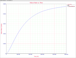
The corresponding plot is given below.

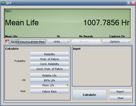
The [math]\displaystyle{ MTTF\,\! }[/math] of the system is obtained by integrating the system's reliability function given by [math]\displaystyle{ {{R}_{s}}(t)=2\cdot {{e}^{-2{{\left( \tfrac{t}{\eta } \right)}^{\beta }}}}+2\cdot {{e}^{-3{{\left( \tfrac{t}{\eta } \right)}^{\beta }}}}-5\cdot {{e}^{-4{{\left( \tfrac{t}{\eta } \right)}^{\beta }}}}+2\cdot {{e}^{-5{{\left( \tfrac{t}{\eta } \right)}^{\beta }}}} }[/math] from time zero to infinity, as given by [math]\displaystyle{ MTTF=\int_{0}^{\infty }{{R}_{s}}\left( t \right)dt \ \,\! }[/math]. Using BlockSim's Analytical QCP, an [math]\displaystyle{ MTTF\,\! }[/math] of 1007.8 hours is calculated, as shown in the figure below.

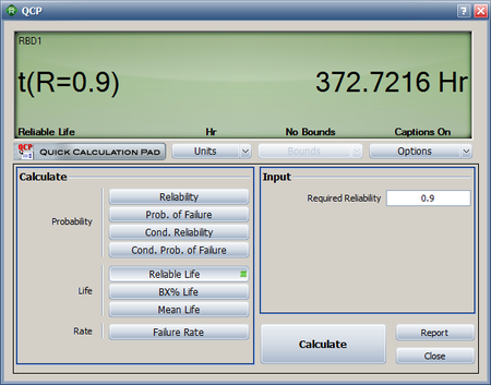
The warranty time can be obtained by solving [math]\displaystyle{ {{R}_{s}}(t)\,\! }[/math] with respect to time for a system reliability [math]\displaystyle{ {{R}_{s}}=0.9\,\! }[/math] . Using the Analytical QCP and selecting the Warranty Time option, a time of 372.72 hours is obtained, as shown in the following figure.

Lastly, the conditional reliability can be obtained using [math]\displaystyle{ R(T,t)=\frac{R(T+t)}{R(T)} }[/math] and [math]\displaystyle{ {{R}_{s}}(t)=2\cdot {{e}^{-2{{\left( \tfrac{t}{\eta } \right)}^{\beta }}}}+2\cdot {{e}^{-3{{\left( \tfrac{t}{\eta } \right)}^{\beta }}}}-5\cdot {{e}^{-4{{\left( \tfrac{t}{\eta } \right)}^{\beta }}}}+2\cdot {{e}^{-5{{\left( \tfrac{t}{\eta } \right)}^{\beta }}}} }[/math], or:

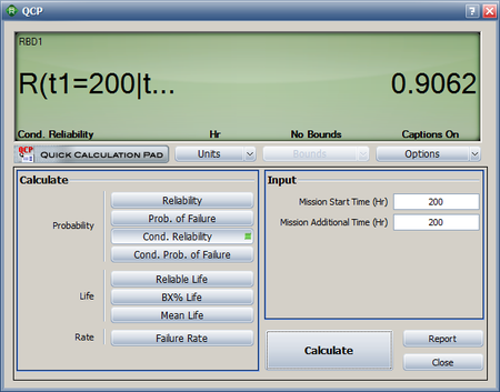
[math]\displaystyle{ \begin{align} R(200,200)= & \frac{R(400)}{R(200)} \\ = & \frac{0.883825}{0.975321} \\ = & 0.906189 \end{align} }[/math]

This can be calculated using BlockSim's Analytical QCP, as shown below.