Weibull++ Examples and Case Studies
Exponential Dstribution for Grouped Data
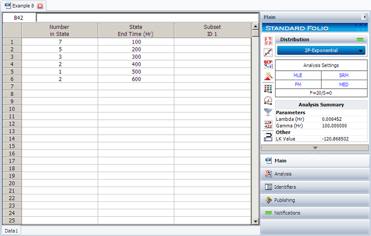
20 units were reliability tested with the following results:
| Table - Life Test Data | |
| Number of Units in Group | Time-to-Failure |
|---|---|
| 7 | 100 |
| 5 | 200 |
| 3 | 300 |
| 2 | 400 |
| 1 | 500 |
| 2 | 600 |
1. Assuming a 2-parameter exponential distribution, estimate the parameters by hand using the MLE analysis method.
2. Repeat the above using Weibull++. (Enter the data as grouped data to duplicate the results.)
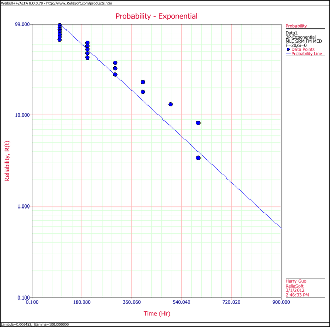
3. Show the Probability plot for the analysis results.
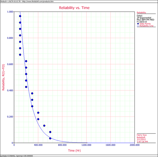
4. Show the Reliability vs. Time plot for the results.
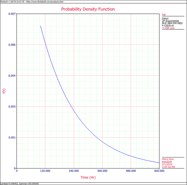
5. Show the pdf plot for the results.
6. Show the Failure Rate vs. Time plot for the results.
7. Estimate the parameters using the rank regression on Y (RRY) analysis method (and using grouped ranks).
Solution
1. For the 2-parameter exponential distribution and for [math]\displaystyle{ \hat{\gamma }=100\,\! }[/math] hours (first failure), the partial of the log-likelihood function, [math]\displaystyle{ \lambda\,\! }[/math], becomes:
- [math]\displaystyle{ \begin{align} \frac{\partial \Lambda }{\partial \lambda }= &\underset{i=1}{\overset{6}{\mathop \sum }}\,{N_i} \left[ \frac{1}{\lambda }-\left( {{T}_{i}}-100 \right) \right]=0\\ \Rightarrow & 7[\frac{1}{\lambda }-(100-100)]+5[\frac{1}{\lambda}-(200-100)] + \ldots +2[\frac{1}{\lambda}-(600-100)]\\ = & 0\\ \Rightarrow & \hat{\lambda}=\frac{20}{3100}=0.0065 \text{fr/hr} \end{align} \,\! }[/math]
2. Enter the data in a Weibull++ standard folio and calculate it as shown next.
3. On the Plot page of the folio, the exponential Probability plot will appear as shown next.
4. View the Reliability vs. Time plot.
5. View the pdf plot.
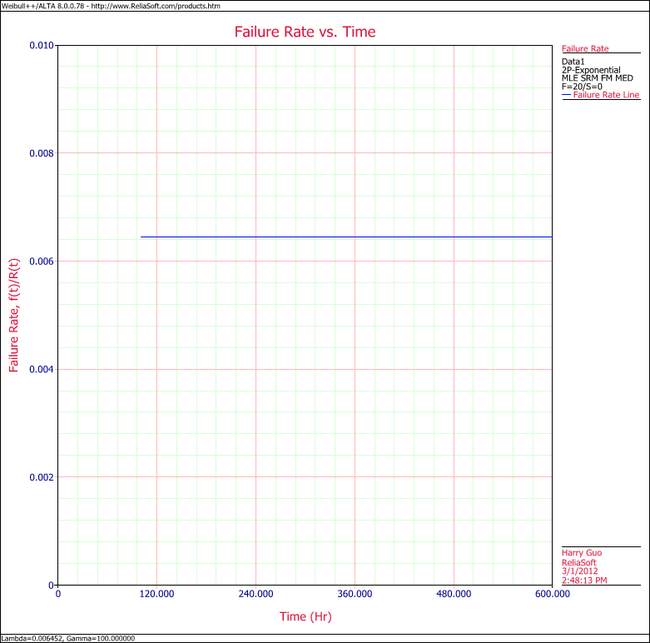
6. View the Failure Rate vs. Time plot.
Note that, as described at the beginning of this chapter, the failure rate for the exponential distribution is constant. Also note that the Failure Rate vs. Time plot does show values for times before the location parameter, [math]\displaystyle{ \gamma \,\! }[/math], at 100 hours.
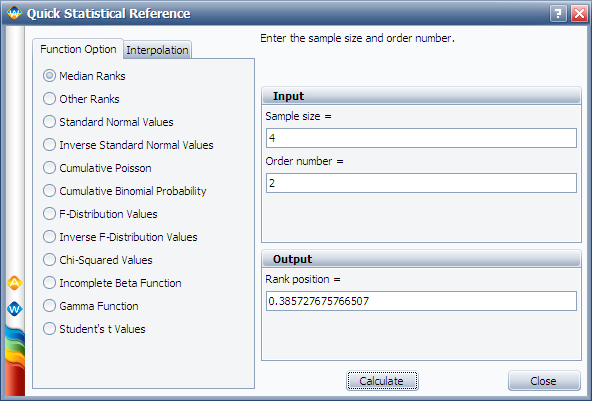
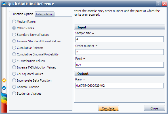
7. In the case of grouped data, one must be cautious when estimating the parameters using a rank regression method. This is because the median rank values are determined from the total number of failures observed by time [math]\displaystyle{ {{T}_{i}}\,\! }[/math] where [math]\displaystyle{ i\,\! }[/math] indicates the group number. In this example, the total number of groups is [math]\displaystyle{ N=6\,\! }[/math] and the total number of units is [math]\displaystyle{ {{N}_{T}}=20\,\! }[/math]. Thus, the median rank values will be estimated for 20 units and for the total failed units ([math]\displaystyle{ {{N}_{{{F}_{i}}}}\,\! }[/math]) up to the [math]\displaystyle{ {{i}^{th}}\,\! }[/math] group, for the [math]\displaystyle{ {{i}^{th}}\,\! }[/math] rank value. The median ranks values can be found from rank tables or they can be estimated using ReliaSoft's Quick Statistical Reference tool.
For example, the median rank value of the fourth group will be the [math]\displaystyle{ {{17}^{th}}\,\! }[/math] rank out of a sample size of twenty units (or 81.945%).
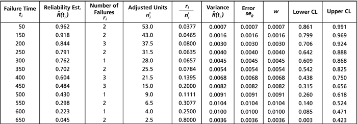
The following table is then constructed.
Given the values in the table above, calculate [math]\displaystyle{ \hat{a}\,\! }[/math] and [math]\displaystyle{ \hat{b}\,\! }[/math]:
- [math]\displaystyle{ \begin{align} & \hat{b}= & \frac{\underset{i=1}{\overset{6}{\mathop{\sum }}}\,{{t}_{i}}{{y}_{i}}-(\underset{i=1}{\overset{6}{\mathop{\sum }}}\,{{t}_{i}})(\underset{i=1}{\overset{6}{\mathop{\sum }}}\,{{y}_{i}})/6}{\underset{i=1}{\overset{6}{\mathop{\sum }}}\,t_{i}^{2}-{{(\underset{i=1}{\overset{6}{\mathop{\sum }}}\,{{t}_{i}})}^{2}}/6} \\ & & \\ & \hat{b}= & \frac{-4320.3362-(2100)(-9.6476)/6}{910,000-{{(2100)}^{2}}/6} \end{align}\,\! }[/math]
or:
- [math]\displaystyle{ \hat{b}=-0.005392\,\! }[/math]
and:
- [math]\displaystyle{ \hat{a}=\overline{y}-\hat{b}\overline{t}=\frac{\underset{i=1}{\overset{N}{\mathop{\sum }}}\,{{y}_{i}}}{N}-\hat{b}\frac{\underset{i=1}{\overset{N}{\mathop{\sum }}}\,{{t}_{i}}}{N}\,\! }[/math]
or:
- [math]\displaystyle{ \hat{a}=\frac{-9.6476}{6}-(-0.005392)\frac{2100}{6}=0.2793\,\! }[/math]
Therefore:
- [math]\displaystyle{ \hat{\lambda }=-\hat{b}=-(-0.005392)=0.05392\text{ failures/hour}\,\! }[/math]
and:
- [math]\displaystyle{ \hat{\gamma }=\frac{\hat{a}}{\hat{\lambda }}=\frac{0.2793}{0.005392}\,\! }[/math]
or:
- [math]\displaystyle{ \hat{\gamma }\simeq 51.8\text{ hours}\,\! }[/math]
Then:
- [math]\displaystyle{ f(T)=(0.005392){{e}^{-0.005392(T-51.8)}}\,\! }[/math]
Using Weibull++, the estimated parameters are:
- [math]\displaystyle{ \begin{align} \hat{\lambda }= & 0.0054\text{ failures/hour} \\ \hat{\gamma }= & 51.82\text{ hours} \end{align}\,\! }[/math]
The small difference in the values from Weibull++ is due to rounding. In the application, the calculations and the rank values are carried out up to the [math]\displaystyle{ 15^{th}\,\! }[/math] decimal point.
Exponential Distribution Auto Batch Run Example
A number of leukemia patients were treated with either drug 6MP or a placebo, and the times in weeks until cancer symptoms returned were recorded. Analyze each treatment separately [21, p.175].
| Table - Leukemia Treatment Results | |||
| Time (weeks) | Number of Patients | Treament | Comments |
|---|---|---|---|
| 1 | 2 | placebo | |
| 2 | 2 | placebo | |
| 3 | 1 | placebo | |
| 4 | 2 | placebo | |
| 5 | 2 | placebo | |
| 6 | 4 | 6MP | 3 patients completed |
| 7 | 1 | 6MP | |
| 8 | 4 | placebo | |
| 9 | 1 | 6MP | Not completed |
| 10 | 2 | 6MP | 1 patient completed |
| 11 | 2 | placebo | |
| 11 | 1 | 6MP | Not completed |
| 12 | 2 | placebo | |
| 13 | 1 | 6MP | |
| 15 | 1 | placebo | |
| 16 | 1 | 6MP | |
| 17 | 1 | placebo | |
| 17 | 1 | 6MP | Not completed |
| 19 | 1 | 6MP | Not completed |
| 20 | 1 | 6MP | Not completed |
| 22 | 1 | placebo | |
| 22 | 1 | 6MP | |
| 23 | 1 | placebo | |
| 23 | 1 | 6MP | |
| 25 | 1 | 6MP | Not completed |
| 32 | 2 | 6MP | Not completed |
| 34 | 1 | 6MP | Not completed |
| 35 | 1 | 6MP | Not completed |
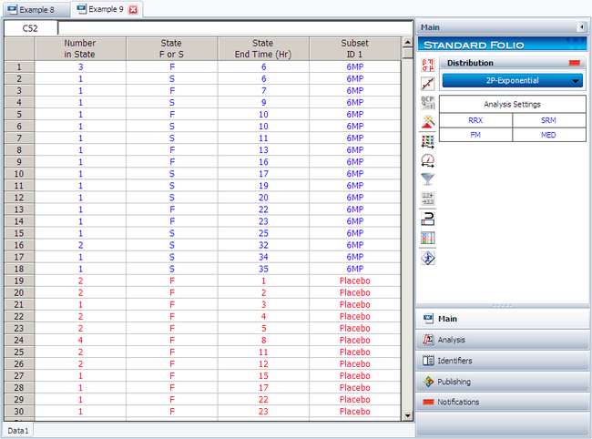
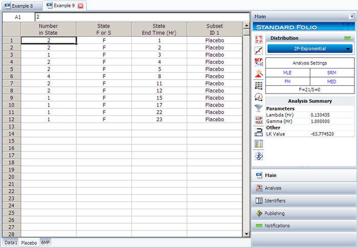
Create a new Weibull++ standard folio that's configured for grouped times-to-failure data with suspensions. In the first column, enter the number of patients. Whenever there are uncompleted tests, enter the number of patients who completed the test separately from the number of patients who did not (e.g., if 4 patients had symptoms return after 6 weeks and only 3 of them completed the test, then enter 1 in one row and 3 in another). In the second column enter F if the patients completed the test and S if they didn't. In the third column enter the time, and in the fourth column (Subset ID) specify whether the 6MP drug or a placebo was used.
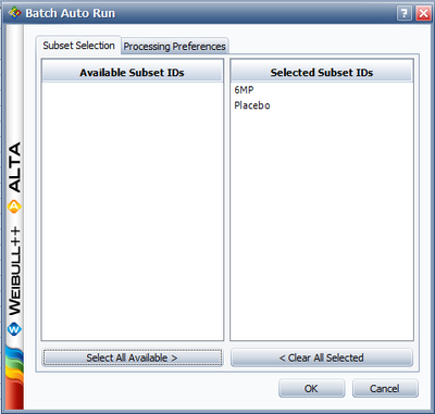
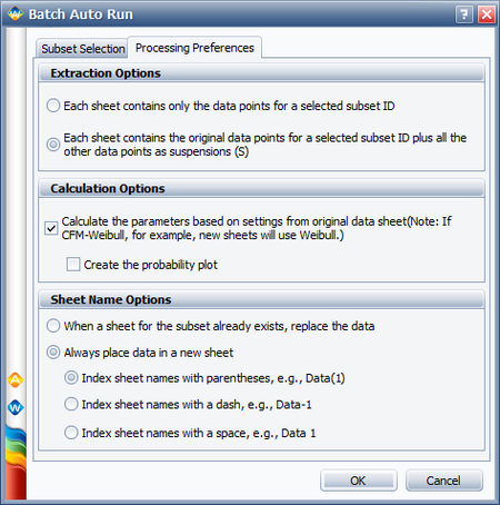
Next, open the Batch Auto Run utility and select to separate the 6MP drug from the placebo, as shown next.
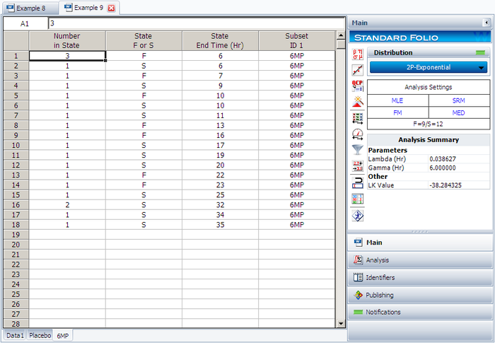
The software will create two data sheets, one for each subset ID, as shown next.
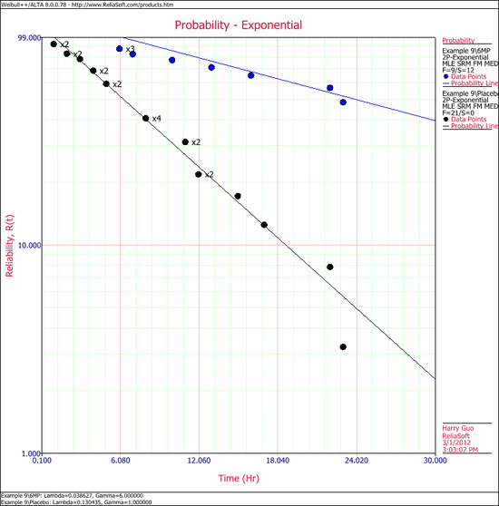
Calculate both data sheets using the 2-parameter exponential distribution and the MLE analysis method, then insert an additional plot and select to show the analysis results for both data sheets on that plot, which will appear as shown next.
Weibull Distribution Examples
Three-parameter Weibull distribution example
Median Rank Plot Example
In this example, we will determine the median rank value used for plotting the 6th failure from a sample size of 10. This example will use Weibull++'s Quick Statistical Reference (QSR) tool to show how the points in the plot of the following example are calculated.
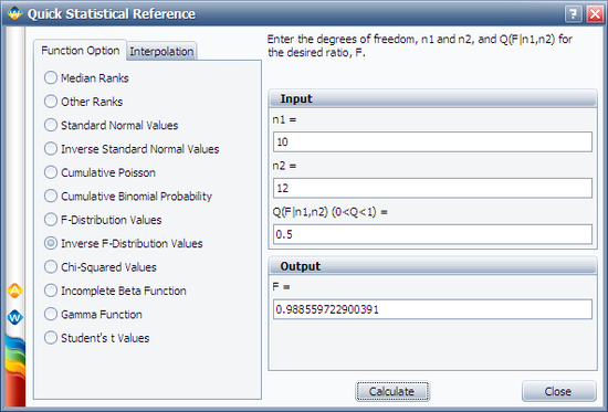
First, open the Quick Statistical Reference tool and select the Inverse F-Distribution Values option.
In this example, n1 = 10, j = 6, m = 2(10 - 6 + 1) = 10, and n2 = 2 x 6 = 12.
Thus, from the F-distribution rank equation:
- [math]\displaystyle{ MR=\frac{1}{1+\left( \frac{10-6+1}{6} \right){{F}_{0.5;10;12}}}\,\! }[/math]
Use the QSR to calculate the value of F0.5;10;12 = 0.9886, as shown next:
Consequently:
- [math]\displaystyle{ MR=\frac{1}{1+\left( \frac{5}{6} \right)\times 0.9886}=0.5483=54.83%\,\! }[/math]
Another method is to use the Median Ranks option directly, which yields MR(%) = 54.8305%, as shown next:
Complete Data Example
Assume that 10 identical units (N = 10) are being reliability tested at the same application and operation stress levels. 6 of these units fail during this test after operating the following numbers of hours, [math]\displaystyle{ {T}_{j}\,\! }[/math]: 150, 105, 83, 123, 64 and 46. The test is stopped at the 6th failure. Find the parameters of the Weibull pdf that represents these data.
Solution
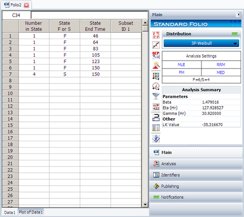
Create a new Weibull++ standard folio that is configured for grouped times-to-failure data with suspensions.
Enter the data in the appropriate columns. Note that there are 4 suspensions, as only 6 of the 10 units were tested to failure (the next figure shows the data as entered). Use the 3-parameter Weibull and MLE for the calculations.
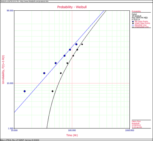
Plot the data.
Note that the original data points, on the curved line, were adjusted by subtracting 30.92 hours to yield a straight line as shown above.
Suspension Data Example
ACME company manufactures widgets, and it is currently engaged in reliability testing a new widget design. 19 units are being reliability tested, but due to the tremendous demand for widgets, units are removed from the test whenever the production cannot cover the demand. The test is terminated at the 67th day when the last widget is removed from the test. The following table contains the collected data.
| Data Point Index | State (F/S) | Time to Failure |
| 1 | F | 2 |
| 2 | S | 3 |
| 3 | F | 5 |
| 4 | S | 7 |
| 5 | F | 11 |
| 6 | S | 13 |
| 7 | S | 17 |
| 8 | S | 19 |
| 9 | F | 23 |
| 10 | F | 29 |
| 11 | S | 31 |
| 12 | F | 37 |
| 13 | S | 41 |
| 14 | F | 43 |
| 15 | S | 47 |
| 16 | S | 53 |
| 17 | F | 59 |
| 18 | S | 61 |
| 19 | S | 67 |
Solution
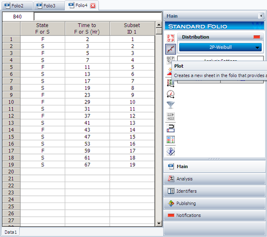
In this example, we see that the number of failures is less than the number of suspensions. This is a very common situation, since reliability tests are often terminated before all units fail due to financial or time constraints. Furthermore, some suspensions will be recorded when a failure occurs that is not due to a legitimate failure mode, such as operator error. In cases such as this, a suspension is recorded, since the unit under test cannot be said to have had a legitimate failure.
Enter the data into a Weibull++ standard folio that is configured for times-to-failure data with suspensions. The folio will appear as shown next:
We will use the 2-parameter Weibull to solve this problem. The parameters using maximum likelihood are:
- [math]\displaystyle{ \begin{align} & \hat{\beta }=1.145 \\ & \hat{\eta }=65.97 \\ \end{align}\,\! }[/math]
Using RRX:
- [math]\displaystyle{ \begin{align} & \hat{\beta }=0.914\\ & \hat{\eta }=79.38 \\ \end{align}\,\! }[/math]
Using RRY:
- [math]\displaystyle{ \begin{align} & \hat{\beta }=0.895\\ & \hat{\eta }=82.02 \\ \end{align}\,\! }[/math]
Interval Data Example
Suppose we have run an experiment with 8 units tested and the following is a table of their last inspection times and failure times:
| Data Point Index | Last Inspection | Failure Time |
| 1 | 30 | 32 |
| 2 | 32 | 35 |
| 3 | 35 | 37 |
| 4 | 37 | 40 |
| 5 | 42 | 42 |
| 6 | 45 | 45 |
| 7 | 50 | 50 |
| 8 | 55 | 55 |
Analyze the data using several different parameter estimation techniques and compare the results.
Solution
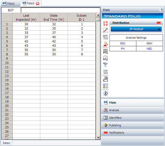
Enter the data into a Weibull++ standard folio that is configured for interval data. The data is entered as follows:
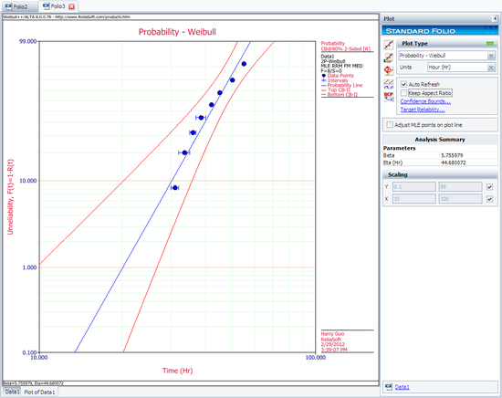
The computed parameters using maximum likelihood are:
- [math]\displaystyle{ \begin{align} & \hat{\beta }=5.76 \\ & \hat{\eta }=44.68 \\ \end{align}\,\! }[/math]
Using RRX or rank regression on X:
- [math]\displaystyle{ \begin{align} & \hat{\beta }=5.70 \\ & \hat{\eta }=44.54 \\ \end{align}\,\! }[/math]
Using RRY or rank regression on Y:
- [math]\displaystyle{ \begin{align} & \hat{\beta }=5.41 \\ & \hat{\eta }=44.76 \\ \end{align}\,\! }[/math]
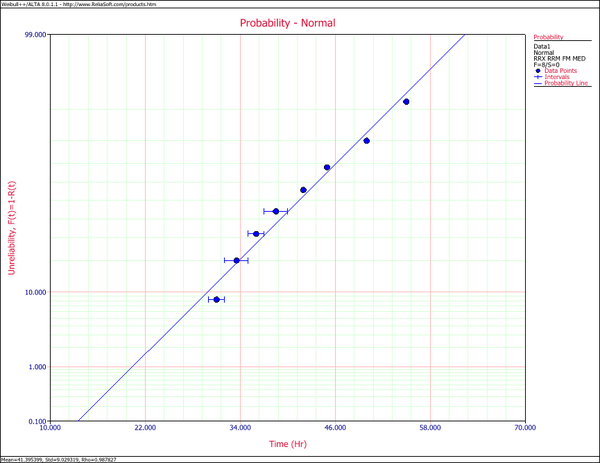
The plot of the MLE solution with the two-sided 90% confidence bounds is:
Mixed Data Types Example
From Dimitri Kececioglu, Reliability & Life Testing Handbook, Page 406. [20].
Estimate the parameters for the 3-parameter Weibull, for a sample of 10 units that are all tested to failure. The recorded failure times are 200; 370; 500; 620; 730; 840; 950; 1,050; 1,160 and 1,400 hours.
Published Results:
Published results (using probability plotting):
- [math]\displaystyle{ {\widehat{\beta}} = 3.0\,\! }[/math], [math]\displaystyle{ {\widehat{\eta}} = 1,220\,\! }[/math], [math]\displaystyle{ {\widehat{\gamma}} = -300\,\! }[/math]
Computed Results in Weibull++
Weibull++ computed parameters for rank regression on X are:
- [math]\displaystyle{ {\widehat{\beta}} = 2.9013\,\! }[/math], [math]\displaystyle{ {\widehat{\eta}} = 1195.5009\,\! }[/math], [math]\displaystyle{ {\widehat{\gamma}} = -279.000\,\! }[/math]
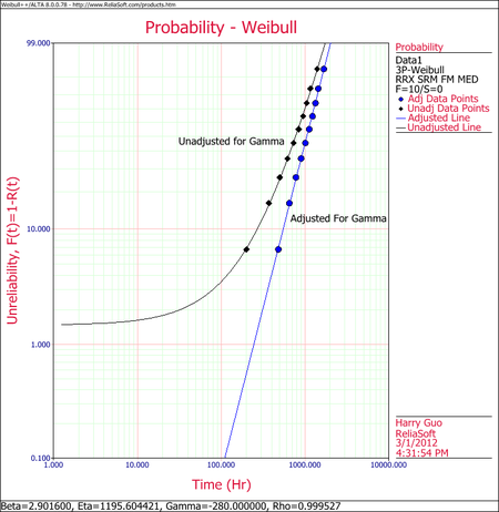
The small difference between the published results and the ones obtained from Weibull++ are due to the difference in the estimation method. In the publication the parameters were estimated using probability plotting (i.e., the fitted line was "eye-balled"). In Weibull++, the parameters were estimated using non-linear regression (a more accurate, mathematically fitted line). Note that γ in this example is negative. This means that the unadjusted for γ line is concave up, as shown next.
Weibull Distribution RRX Example
Assume that 6 identical units are being tested. The failure times are: 93, 34, 16, 120, 53 and 75 hours.
1. What is the unreliability of the units for a mission duration of 30 hours, starting the mission at age zero?
2. What is the reliability for a mission duration of 10 hours, starting the new mission at the age of T = 30 hours?
3. What is the longest mission that this product should undertake for a reliability of 90%?
Solution
1. First, we use Weibull++ to obtain the parameters using RRX.
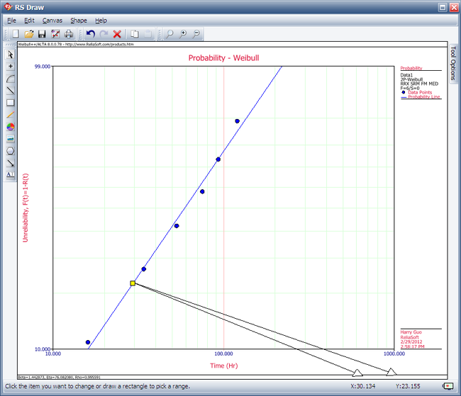
Then, we investigate several methods of solution for this problem. The first, and more laborious, method is to extract the information directly from the plot. You may do this with either the screen plot in RS Draw or the printed copy of the plot. (When extracting information from the screen plot in RS Draw, note that the translated axis position of your mouse is always shown on the bottom right corner.)
Using this first method, enter either the screen plot or the printed plot with T = 30 hours, go up vertically to the straight line fitted to the data, then go horizontally to the ordinate, and read off the result. A good estimate of the unreliability is 23%. (Also, the reliability estimate is 1.0 - 0.23 = 0.77 or 77%.)
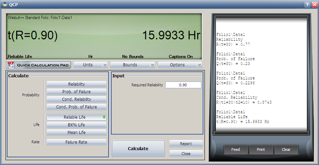
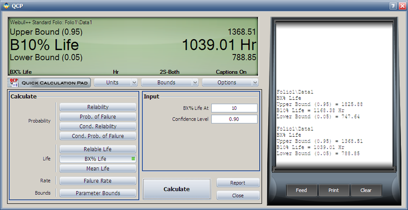
The second method involves the use of the Quick Calculation Pad (QCP).
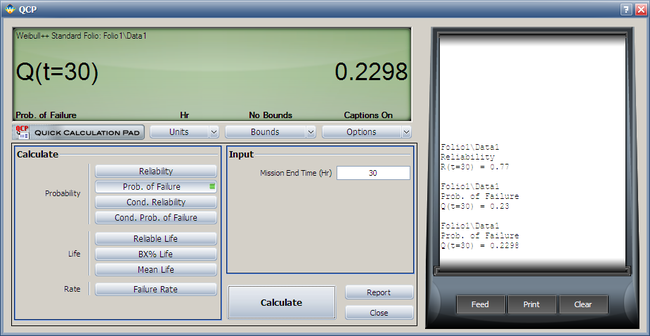
Select the Prob. of Failure calculation option and enter 30 hours in the Mission End Time field.
Note that the results in QCP vary according to the parameter estimation method used. The above results are obtained using RRX.
2. The conditional reliability is given by:
- [math]\displaystyle{ R(t|T)=\frac{R(T+t)}{R(T)}\,\! }[/math]
or:
- [math]\displaystyle{ \hat{R}(10hr|30hr)=\frac{\hat{R}(10+30)}{\hat{R}(30)}=\frac{\hat{R}(40)}{\hat{R}(30)}\,\! }[/math]
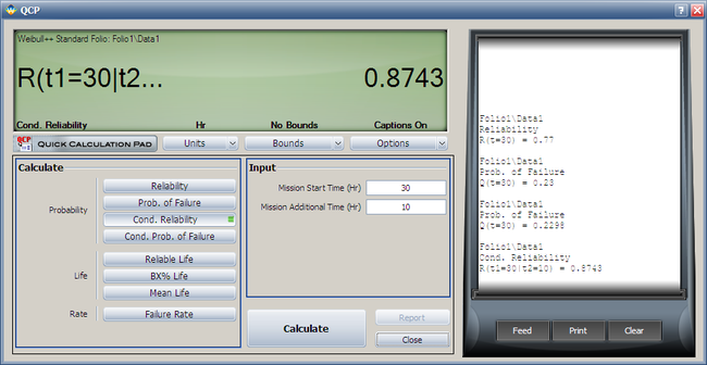
Again, the QCP can provide this result directly and more accurately than the plot.
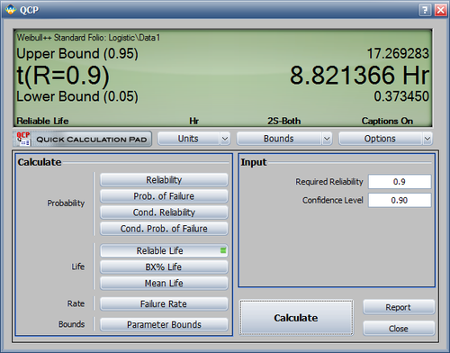
3. To use the QCP to solve for the longest mission that this product should undertake for a reliability of 90%, choose Reliable Life and enter 0.9 for the required reliability. The result is 15.9933 hours.
Benchmark with Published Examples
The following examples compare published results to computed results obtained with Weibull++.
Complete Data RRY Example
From Dimitri Kececioglu, Reliability & Life Testing Handbook, Page 418 [20].
Sample of 10 units, all tested to failure. The failures were recorded at 16, 34, 53, 75, 93, 120, 150, 191, 240 and 339 hours.
Published Results
Published Results (using Rank Regression on Y):
- [math]\displaystyle{ \begin{align} & \widehat{\beta }=1.20 \\ & \widehat{\eta} = 146.2 \\ & \hat{\rho }=0.998703\\ \end{align}\,\! }[/math]
Computed Results in Weibull++
This same data set can be entered into a Weibull++ standard data sheet. Use RRY for the estimation method.
Weibull++ computed parameters for RRY are:
- [math]\displaystyle{ \begin{align} & \widehat{\beta }=1.1973 \\ & \widehat{\eta} = 146.2545 \\ & \hat{\rho }=0.9999\\ \end{align}\,\! }[/math]
The small difference between the published results and the ones obtained from Weibull++ is due to the difference in the median rank values between the two (in the publication, median ranks are obtained from tables to 3 decimal places, whereas in Weibull++ they are calculated and carried out up to the 15th decimal point).
You will also notice that in the examples that follow, a small difference may exist between the published results and the ones obtained from Weibull++. This can be attributed to the difference between the computer numerical precision employed by Weibull++ and the lower number of significant digits used by the original authors. In most of these publications, no information was given as to the numerical precision used.
Suspension Data MLE Example
From Wayne Nelson, Fan Example, Applied Life Data Analysis, page 317 [30].
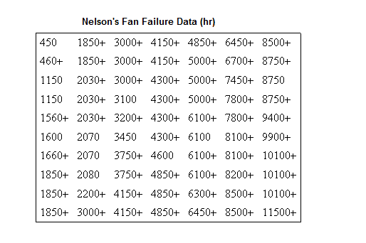
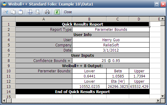
70 diesel engine fans accumulated 344,440 hours in service and 12 of them failed. A table of their life data is shown next (+ denotes non-failed units or suspensions, using Dr. Nelson's nomenclature). Evaluate the parameters with their two-sided 95% confidence bounds, using MLE for the 2-parameter Weibull distribution.
Published Results:
Weibull parameters (2P-Weibull, MLE):
- [math]\displaystyle{ \begin{align} & \widehat{\beta }=1.0584 \\ & \widehat{\eta} = 26,296 \\ \end{align}\,\! }[/math]
Published 95% FM confidence limits on the parameters:
- [math]\displaystyle{ \begin{align} & \widehat{\beta }=\lbrace 0.6441, \text{ }1.7394\rbrace \\ & \widehat{\eta} = \lbrace 10,522, \text{ }65,532\rbrace \\ \end{align}\,\! }[/math]
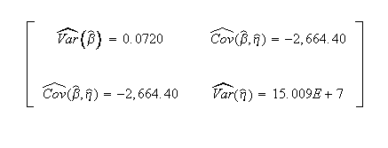
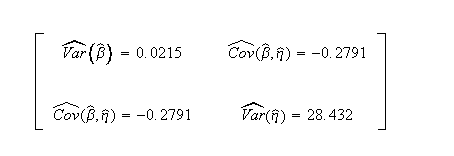
Published variance/covariance matrix:
Note that Nelson expresses the results as multiples of 1,000 (or = 26.297, etc.). The published results were adjusted by this factor to correlate with Weibull++ results.
Computed Results in Weibull++
This same data set can be entered into a Weibull++ standard folio, using 2-parameter Weibull and MLE to calculate the parameter estimates.
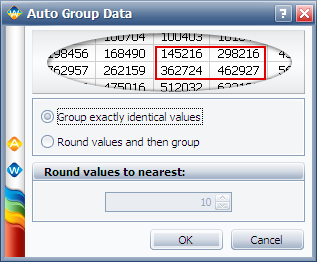
You can also enter the data as given in table without grouping them by opening a data sheet configured for suspension data. Then click the Group Data icon and chose Group exactly identical values.
The data will be automatically grouped and put into a new grouped data sheet.
Weibull++ computed parameters for maximum likelihood are:
- [math]\displaystyle{ \begin{align} & \widehat{\beta }=1.0584 \\ & \widehat{\eta} = 26,297 \\ \end{align}\,\! }[/math]
Weibull++ computed 95% FM confidence limits on the parameters:
- [math]\displaystyle{ \begin{align} & \widehat{\beta }=\lbrace 0.6441, \text{ }1.7394\rbrace \\ & \widehat{\eta} = \lbrace 10,522, \text{ }65,532\rbrace \\ \end{align}\,\! }[/math]
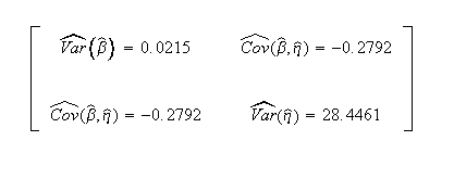
Weibull++ computed/variance covariance matrix:
The two-sided 95% bounds on the parameters can be determined from the QCP. Calculate and then click Report to see the results.
Interval Data MLE Example
From Wayne Nelson, Applied Life Data Analysis, Page 415 [30]. 167 identical parts were inspected for cracks. The following is a table of their last inspection times and times-to-failure:
Published Results:
Published results (using MLE):
- [math]\displaystyle{ \begin{align} & \widehat{\beta }=1.486 \\ & \widehat{\eta} = 71.687\\ \end{align}\,\! }[/math]
Published 95% FM confidence limits on the parameters:
- [math]\displaystyle{ \begin{align} & \widehat{\beta }=\lbrace 1.224, \text{ }1.802\rbrace \\ & \widehat{\eta} = \lbrace 61.962, \text{ }82.938\rbrace \\ \end{align}\,\! }[/math]
Published variance/covariance matrix:
Computed Results in Weibull++
This same data set can be entered into a Weibull++ standard folio that's configured for grouped times-to-failure data with suspensions and interval data.
Weibull++ computed parameters for maximum likelihood are:
- [math]\displaystyle{ \begin{align} & \widehat{\beta }=1.485 \\ & \widehat{\eta} = 71.690\\ \end{align}\,\! }[/math]
Weibull++ computed 95% FM confidence limits on the parameters:
- [math]\displaystyle{ \begin{align} & \widehat{\beta }=\lbrace 1.224, \text{ }1.802\rbrace \\ & \widehat{\eta} = \lbrace 61.961, \text{ }82.947\rbrace \\ \end{align}\,\! }[/math]
Weibull++ computed/variance covariance matrix:
Grouped Suspension MLE Example
From Dallas R. Wingo, IEEE Transactions on Reliability Vol. R-22, No 2, June 1973, Pages 96-100.
Wingo uses the following times-to-failure: 37, 55, 64, 72, 74, 87, 88, 89, 91, 92, 94, 95, 97, 98, 100, 101, 102, 102, 105, 105, 107, 113, 117, 120, 120, 120, 122, 124, 126, 130, 135, 138, 182. In addition, the following suspensions are used: 4 at 70, 5 at 80, 4 at 99, 3 at 121 and 1 at 150.
Published Results (using MLE)
- [math]\displaystyle{ \begin{align} & \widehat{\beta }=3.7596935\\ & \widehat{\eta} = 106.49758 \\ & \hat{\gamma }=14.451684\\ \end{align}\,\! }[/math]
Computed Results in Weibull++
- [math]\displaystyle{ \begin{align} & \widehat{\beta }=3.7596935\\ & \widehat{\eta} = 106.49758 \\ & \hat{\gamma }=14.451684\\ \end{align}\,\! }[/math]
Note that you must select the Use True 3-P MLEoption in the Weibull++ Application Setup to replicate these results.
3-P Probability Plot Example
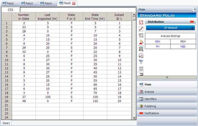
Suppose we want to model a left censored, right censored, interval, and complete data set, consisting of 274 units under test of which 185 units fail. The following table contains the data.
| Data Point Index | Number in State | Last Inspection | State (S or F) | State End Time |
| 1 | 2 | 5 | F | 5 |
| 2 | 23 | 5 | S | 5 |
| 3 | 28 | 0 | F | 7 |
| 4 | 4 | 10 | F | 10 |
| 5 | 7 | 15 | F | 15 |
| 6 | 8 | 20 | F | 20 |
| 7 | 29 | 20 | S | 20 |
| 8 | 32 | 0 | F | 22 |
| 9 | 6 | 25 | F | 25 |
| 10 | 4 | 27 | F | 30 |
| 11 | 8 | 30 | F | 35 |
| 12 | 5 | 30 | F | 40 |
| 13 | 9 | 27 | F | 45 |
| 14 | 7 | 25 | F | 50 |
| 15 | 5 | 20 | F | 55 |
| 16 | 3 | 15 | F | 60 |
| 17 | 6 | 10 | F | 65 |
| 18 | 3 | 5 | F | 70 |
| 19 | 37 | 100 | S | 100 |
| 20 | 48 | 0 | F | 102 |
Solution
Since standard ranking methods for dealing with these different data types are inadequate, we will want to use the ReliaSoft ranking method. This option is the default in Weibull++ when dealing with interval data. The filled-out standard folio is shown next:
The computed parameters using MLE are:
- [math]\displaystyle{ \hat{\beta }=0.748;\text{ }\hat{\eta }=44.38\,\! }[/math]
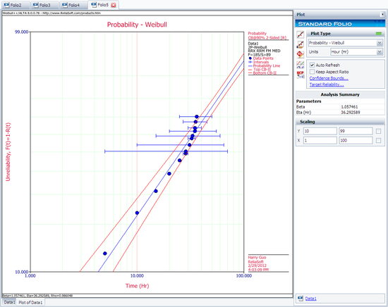
Using RRX:
- [math]\displaystyle{ \hat{\beta }=1.057;\text{ }\hat{\eta }=36.29\,\! }[/math]
Using RRY:
- [math]\displaystyle{ \hat{\beta }=0.998;\text{ }\hat{\eta }=37.16\,\! }[/math]
The plot with the two-sided 90% confidence bounds for the rank regression on X solution is:
Weibull-Bayesian with Lognormal Prior Example
A manufacturer has tested prototypes of a modified product. The test was terminated at 2,000 hours, with only 2 failures observed from a sample size of 18. The following table shows the data.
| Number of State | State of F or S | State End Time |
|---|---|---|
| 1 | F | 1180 |
| 1 | F | 1842 |
| 16 | S | 2000 |
Because of the lack of failure data in the prototype testing, the manufacturer decided to use information gathered from prior tests on this product to increase the confidence in the results of the prototype testing. This decision was made because failure analysis indicated that the failure mode of the two failures is the same as the one that was observed in previous tests. In other words, it is expected that the shape of the distribution (beta) hasn't changed, but hopefully the scale (eta) has, indicating longer life. The 2-parameter Weibull distribution was used to model all prior tests results. The estimated beta ([math]\displaystyle{ \beta\,\! }[/math]) parameters of the prior test results are as follows:
| Betas Obtained for Similar Mode |
|---|
| 1.7 |
| 2.1 |
| 2.4 |
| 3.1 |
| 3.5 |
Solution
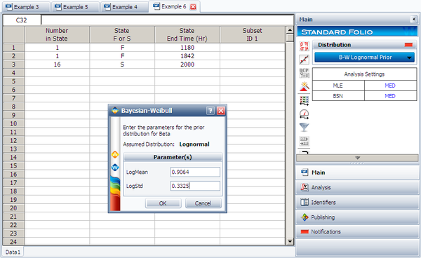
First, in order to fit the data to a Bayesian-Weibull model, a prior distribution for beta needs to be determined. Based on the beta values in the prior tests, the prior distribution for beta is found to be a lognormal distribution with [math]\displaystyle{ \mu = 0.9064\,\! }[/math], [math]\displaystyle{ \sigma = 0.3325\,\! }[/math]. (The values of the parameters can be obtained by entering the beta values into a Weibull++ standard folio and analyzing it using the lognormal distribution and the RRX analysis method.)
Next, enter the data from the prototype testing into a standard folio. On the control panel, choose the Bayesian-Weibull > B-W Lognormal Prior distribution. Click Calculate and enter the parameters of the lognormal distribution, as shown next.
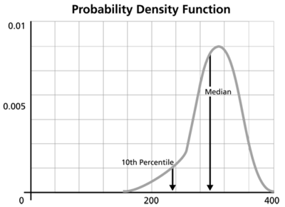
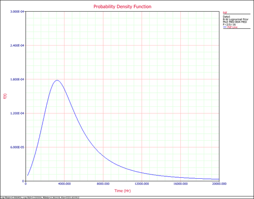
Click OK. The result is Beta (Median) = 2.361219 and Eta (Median) = 5321.631912 (by default Weibull++ returns the median values of the posterior distribution). Suppose that the reliability at 3,000 hours is the metric of interest in this example. Using the QCP, the reliability is calculated to be 76.97% at 3,000 hours. The following picture depicts the posterior pdf plot of the reliability at 3,000, with the corresponding median value as well as the 10th percentile value. The 10th percentile constitutes the 90% lower 1-sided bound on the reliability at 3,000 hours, which is calculated to be 50.77%.
The pdf of the times-to-failure data can be plotted in Weibull++, as shown next:
Median Rank Plot Example
Median Rank Plot Example
In this example, we will determine the median rank value used for plotting the 6th failure from a sample size of 10. This example will use Weibull++'s Quick Statistical Reference (QSR) tool to show how the points in the plot of the following example are calculated.
First, open the Quick Statistical Reference tool and select the Inverse F-Distribution Values option.
In this example, n1 = 10, j = 6, m = 2(10 - 6 + 1) = 10, and n2 = 2 x 6 = 12.
Thus, from the F-distribution rank equation:
- [math]\displaystyle{ MR=\frac{1}{1+\left( \frac{10-6+1}{6} \right){{F}_{0.5;10;12}}}\,\! }[/math]
Use the QSR to calculate the value of F0.5;10;12 = 0.9886, as shown next:
Consequently:
- [math]\displaystyle{ MR=\frac{1}{1+\left( \frac{5}{6} \right)\times 0.9886}=0.5483=54.83%\,\! }[/math]
Another method is to use the Median Ranks option directly, which yields MR(%) = 54.8305%, as shown next:
Complete Data Example
Assume that 10 identical units (N = 10) are being reliability tested at the same application and operation stress levels. 6 of these units fail during this test after operating the following numbers of hours, [math]\displaystyle{ {T}_{j}\,\! }[/math]: 150, 105, 83, 123, 64 and 46. The test is stopped at the 6th failure. Find the parameters of the Weibull pdf that represents these data.
Solution
Create a new Weibull++ standard folio that is configured for grouped times-to-failure data with suspensions.
Enter the data in the appropriate columns. Note that there are 4 suspensions, as only 6 of the 10 units were tested to failure (the next figure shows the data as entered). Use the 3-parameter Weibull and MLE for the calculations.
Plot the data.
Note that the original data points, on the curved line, were adjusted by subtracting 30.92 hours to yield a straight line as shown above.
Suspension Data Example
ACME company manufactures widgets, and it is currently engaged in reliability testing a new widget design. 19 units are being reliability tested, but due to the tremendous demand for widgets, units are removed from the test whenever the production cannot cover the demand. The test is terminated at the 67th day when the last widget is removed from the test. The following table contains the collected data.
| Data Point Index | State (F/S) | Time to Failure |
| 1 | F | 2 |
| 2 | S | 3 |
| 3 | F | 5 |
| 4 | S | 7 |
| 5 | F | 11 |
| 6 | S | 13 |
| 7 | S | 17 |
| 8 | S | 19 |
| 9 | F | 23 |
| 10 | F | 29 |
| 11 | S | 31 |
| 12 | F | 37 |
| 13 | S | 41 |
| 14 | F | 43 |
| 15 | S | 47 |
| 16 | S | 53 |
| 17 | F | 59 |
| 18 | S | 61 |
| 19 | S | 67 |
Solution
In this example, we see that the number of failures is less than the number of suspensions. This is a very common situation, since reliability tests are often terminated before all units fail due to financial or time constraints. Furthermore, some suspensions will be recorded when a failure occurs that is not due to a legitimate failure mode, such as operator error. In cases such as this, a suspension is recorded, since the unit under test cannot be said to have had a legitimate failure.
Enter the data into a Weibull++ standard folio that is configured for times-to-failure data with suspensions. The folio will appear as shown next:
We will use the 2-parameter Weibull to solve this problem. The parameters using maximum likelihood are:
- [math]\displaystyle{ \begin{align} & \hat{\beta }=1.145 \\ & \hat{\eta }=65.97 \\ \end{align}\,\! }[/math]
Using RRX:
- [math]\displaystyle{ \begin{align} & \hat{\beta }=0.914\\ & \hat{\eta }=79.38 \\ \end{align}\,\! }[/math]
Using RRY:
- [math]\displaystyle{ \begin{align} & \hat{\beta }=0.895\\ & \hat{\eta }=82.02 \\ \end{align}\,\! }[/math]
Interval Data Example
Suppose we have run an experiment with 8 units tested and the following is a table of their last inspection times and failure times:
| Data Point Index | Last Inspection | Failure Time |
| 1 | 30 | 32 |
| 2 | 32 | 35 |
| 3 | 35 | 37 |
| 4 | 37 | 40 |
| 5 | 42 | 42 |
| 6 | 45 | 45 |
| 7 | 50 | 50 |
| 8 | 55 | 55 |
Analyze the data using several different parameter estimation techniques and compare the results.
Solution
Enter the data into a Weibull++ standard folio that is configured for interval data. The data is entered as follows:
The computed parameters using maximum likelihood are:
- [math]\displaystyle{ \begin{align} & \hat{\beta }=5.76 \\ & \hat{\eta }=44.68 \\ \end{align}\,\! }[/math]
Using RRX or rank regression on X:
- [math]\displaystyle{ \begin{align} & \hat{\beta }=5.70 \\ & \hat{\eta }=44.54 \\ \end{align}\,\! }[/math]
Using RRY or rank regression on Y:
- [math]\displaystyle{ \begin{align} & \hat{\beta }=5.41 \\ & \hat{\eta }=44.76 \\ \end{align}\,\! }[/math]
The plot of the MLE solution with the two-sided 90% confidence bounds is:
Mixed Data Types Example
From Dimitri Kececioglu, Reliability & Life Testing Handbook, Page 406. [20].
Estimate the parameters for the 3-parameter Weibull, for a sample of 10 units that are all tested to failure. The recorded failure times are 200; 370; 500; 620; 730; 840; 950; 1,050; 1,160 and 1,400 hours.
Published Results:
Published results (using probability plotting):
- [math]\displaystyle{ {\widehat{\beta}} = 3.0\,\! }[/math], [math]\displaystyle{ {\widehat{\eta}} = 1,220\,\! }[/math], [math]\displaystyle{ {\widehat{\gamma}} = -300\,\! }[/math]
Computed Results in Weibull++
Weibull++ computed parameters for rank regression on X are:
- [math]\displaystyle{ {\widehat{\beta}} = 2.9013\,\! }[/math], [math]\displaystyle{ {\widehat{\eta}} = 1195.5009\,\! }[/math], [math]\displaystyle{ {\widehat{\gamma}} = -279.000\,\! }[/math]
The small difference between the published results and the ones obtained from Weibull++ are due to the difference in the estimation method. In the publication the parameters were estimated using probability plotting (i.e., the fitted line was "eye-balled"). In Weibull++, the parameters were estimated using non-linear regression (a more accurate, mathematically fitted line). Note that γ in this example is negative. This means that the unadjusted for γ line is concave up, as shown next.
Weibull Distribution RRX Example
Assume that 6 identical units are being tested. The failure times are: 93, 34, 16, 120, 53 and 75 hours.
1. What is the unreliability of the units for a mission duration of 30 hours, starting the mission at age zero?
2. What is the reliability for a mission duration of 10 hours, starting the new mission at the age of T = 30 hours?
3. What is the longest mission that this product should undertake for a reliability of 90%?
Solution
1. First, we use Weibull++ to obtain the parameters using RRX.
Then, we investigate several methods of solution for this problem. The first, and more laborious, method is to extract the information directly from the plot. You may do this with either the screen plot in RS Draw or the printed copy of the plot. (When extracting information from the screen plot in RS Draw, note that the translated axis position of your mouse is always shown on the bottom right corner.)
Using this first method, enter either the screen plot or the printed plot with T = 30 hours, go up vertically to the straight line fitted to the data, then go horizontally to the ordinate, and read off the result. A good estimate of the unreliability is 23%. (Also, the reliability estimate is 1.0 - 0.23 = 0.77 or 77%.)
The second method involves the use of the Quick Calculation Pad (QCP).
Select the Prob. of Failure calculation option and enter 30 hours in the Mission End Time field.
Note that the results in QCP vary according to the parameter estimation method used. The above results are obtained using RRX.
2. The conditional reliability is given by:
- [math]\displaystyle{ R(t|T)=\frac{R(T+t)}{R(T)}\,\! }[/math]
or:
- [math]\displaystyle{ \hat{R}(10hr|30hr)=\frac{\hat{R}(10+30)}{\hat{R}(30)}=\frac{\hat{R}(40)}{\hat{R}(30)}\,\! }[/math]
Again, the QCP can provide this result directly and more accurately than the plot.
3. To use the QCP to solve for the longest mission that this product should undertake for a reliability of 90%, choose Reliable Life and enter 0.9 for the required reliability. The result is 15.9933 hours.
Benchmark with Published Examples
The following examples compare published results to computed results obtained with Weibull++.
Complete Data RRY Example
From Dimitri Kececioglu, Reliability & Life Testing Handbook, Page 418 [20].
Sample of 10 units, all tested to failure. The failures were recorded at 16, 34, 53, 75, 93, 120, 150, 191, 240 and 339 hours.
Published Results
Published Results (using Rank Regression on Y):
- [math]\displaystyle{ \begin{align} & \widehat{\beta }=1.20 \\ & \widehat{\eta} = 146.2 \\ & \hat{\rho }=0.998703\\ \end{align}\,\! }[/math]
Computed Results in Weibull++
This same data set can be entered into a Weibull++ standard data sheet. Use RRY for the estimation method.
Weibull++ computed parameters for RRY are:
- [math]\displaystyle{ \begin{align} & \widehat{\beta }=1.1973 \\ & \widehat{\eta} = 146.2545 \\ & \hat{\rho }=0.9999\\ \end{align}\,\! }[/math]
The small difference between the published results and the ones obtained from Weibull++ is due to the difference in the median rank values between the two (in the publication, median ranks are obtained from tables to 3 decimal places, whereas in Weibull++ they are calculated and carried out up to the 15th decimal point).
You will also notice that in the examples that follow, a small difference may exist between the published results and the ones obtained from Weibull++. This can be attributed to the difference between the computer numerical precision employed by Weibull++ and the lower number of significant digits used by the original authors. In most of these publications, no information was given as to the numerical precision used.
Suspension Data MLE Example
From Wayne Nelson, Fan Example, Applied Life Data Analysis, page 317 [30].
70 diesel engine fans accumulated 344,440 hours in service and 12 of them failed. A table of their life data is shown next (+ denotes non-failed units or suspensions, using Dr. Nelson's nomenclature). Evaluate the parameters with their two-sided 95% confidence bounds, using MLE for the 2-parameter Weibull distribution.
Published Results:
Weibull parameters (2P-Weibull, MLE):
- [math]\displaystyle{ \begin{align} & \widehat{\beta }=1.0584 \\ & \widehat{\eta} = 26,296 \\ \end{align}\,\! }[/math]
Published 95% FM confidence limits on the parameters:
- [math]\displaystyle{ \begin{align} & \widehat{\beta }=\lbrace 0.6441, \text{ }1.7394\rbrace \\ & \widehat{\eta} = \lbrace 10,522, \text{ }65,532\rbrace \\ \end{align}\,\! }[/math]
Published variance/covariance matrix:
Note that Nelson expresses the results as multiples of 1,000 (or = 26.297, etc.). The published results were adjusted by this factor to correlate with Weibull++ results.
Computed Results in Weibull++
This same data set can be entered into a Weibull++ standard folio, using 2-parameter Weibull and MLE to calculate the parameter estimates.
You can also enter the data as given in table without grouping them by opening a data sheet configured for suspension data. Then click the Group Data icon and chose Group exactly identical values.
The data will be automatically grouped and put into a new grouped data sheet.
Weibull++ computed parameters for maximum likelihood are:
- [math]\displaystyle{ \begin{align} & \widehat{\beta }=1.0584 \\ & \widehat{\eta} = 26,297 \\ \end{align}\,\! }[/math]
Weibull++ computed 95% FM confidence limits on the parameters:
- [math]\displaystyle{ \begin{align} & \widehat{\beta }=\lbrace 0.6441, \text{ }1.7394\rbrace \\ & \widehat{\eta} = \lbrace 10,522, \text{ }65,532\rbrace \\ \end{align}\,\! }[/math]
Weibull++ computed/variance covariance matrix:
The two-sided 95% bounds on the parameters can be determined from the QCP. Calculate and then click Report to see the results.
Interval Data MLE Example
From Wayne Nelson, Applied Life Data Analysis, Page 415 [30]. 167 identical parts were inspected for cracks. The following is a table of their last inspection times and times-to-failure:
Published Results:
Published results (using MLE):
- [math]\displaystyle{ \begin{align} & \widehat{\beta }=1.486 \\ & \widehat{\eta} = 71.687\\ \end{align}\,\! }[/math]
Published 95% FM confidence limits on the parameters:
- [math]\displaystyle{ \begin{align} & \widehat{\beta }=\lbrace 1.224, \text{ }1.802\rbrace \\ & \widehat{\eta} = \lbrace 61.962, \text{ }82.938\rbrace \\ \end{align}\,\! }[/math]
Published variance/covariance matrix:
Computed Results in Weibull++
This same data set can be entered into a Weibull++ standard folio that's configured for grouped times-to-failure data with suspensions and interval data.
Weibull++ computed parameters for maximum likelihood are:
- [math]\displaystyle{ \begin{align} & \widehat{\beta }=1.485 \\ & \widehat{\eta} = 71.690\\ \end{align}\,\! }[/math]
Weibull++ computed 95% FM confidence limits on the parameters:
- [math]\displaystyle{ \begin{align} & \widehat{\beta }=\lbrace 1.224, \text{ }1.802\rbrace \\ & \widehat{\eta} = \lbrace 61.961, \text{ }82.947\rbrace \\ \end{align}\,\! }[/math]
Weibull++ computed/variance covariance matrix:
Grouped Suspension MLE Example
From Dallas R. Wingo, IEEE Transactions on Reliability Vol. R-22, No 2, June 1973, Pages 96-100.
Wingo uses the following times-to-failure: 37, 55, 64, 72, 74, 87, 88, 89, 91, 92, 94, 95, 97, 98, 100, 101, 102, 102, 105, 105, 107, 113, 117, 120, 120, 120, 122, 124, 126, 130, 135, 138, 182. In addition, the following suspensions are used: 4 at 70, 5 at 80, 4 at 99, 3 at 121 and 1 at 150.
Published Results (using MLE)
- [math]\displaystyle{ \begin{align} & \widehat{\beta }=3.7596935\\ & \widehat{\eta} = 106.49758 \\ & \hat{\gamma }=14.451684\\ \end{align}\,\! }[/math]
Computed Results in Weibull++
- [math]\displaystyle{ \begin{align} & \widehat{\beta }=3.7596935\\ & \widehat{\eta} = 106.49758 \\ & \hat{\gamma }=14.451684\\ \end{align}\,\! }[/math]
Note that you must select the Use True 3-P MLEoption in the Weibull++ Application Setup to replicate these results.
3-P Probability Plot Example
Suppose we want to model a left censored, right censored, interval, and complete data set, consisting of 274 units under test of which 185 units fail. The following table contains the data.
| Data Point Index | Number in State | Last Inspection | State (S or F) | State End Time |
| 1 | 2 | 5 | F | 5 |
| 2 | 23 | 5 | S | 5 |
| 3 | 28 | 0 | F | 7 |
| 4 | 4 | 10 | F | 10 |
| 5 | 7 | 15 | F | 15 |
| 6 | 8 | 20 | F | 20 |
| 7 | 29 | 20 | S | 20 |
| 8 | 32 | 0 | F | 22 |
| 9 | 6 | 25 | F | 25 |
| 10 | 4 | 27 | F | 30 |
| 11 | 8 | 30 | F | 35 |
| 12 | 5 | 30 | F | 40 |
| 13 | 9 | 27 | F | 45 |
| 14 | 7 | 25 | F | 50 |
| 15 | 5 | 20 | F | 55 |
| 16 | 3 | 15 | F | 60 |
| 17 | 6 | 10 | F | 65 |
| 18 | 3 | 5 | F | 70 |
| 19 | 37 | 100 | S | 100 |
| 20 | 48 | 0 | F | 102 |
Solution
Since standard ranking methods for dealing with these different data types are inadequate, we will want to use the ReliaSoft ranking method. This option is the default in Weibull++ when dealing with interval data. The filled-out standard folio is shown next:
The computed parameters using MLE are:
- [math]\displaystyle{ \hat{\beta }=0.748;\text{ }\hat{\eta }=44.38\,\! }[/math]
Using RRX:
- [math]\displaystyle{ \hat{\beta }=1.057;\text{ }\hat{\eta }=36.29\,\! }[/math]
Using RRY:
- [math]\displaystyle{ \hat{\beta }=0.998;\text{ }\hat{\eta }=37.16\,\! }[/math]
The plot with the two-sided 90% confidence bounds for the rank regression on X solution is:
Weibull Disribution Unreliability RRX Example
Assume that 6 identical units are being tested. The failure times are: 93, 34, 16, 120, 53 and 75 hours.
1. What is the unreliability of the units for a mission duration of 30 hours, starting the mission at age zero?
2. What is the reliability for a mission duration of 10 hours, starting the new mission at the age of T = 30 hours?
3. What is the longest mission that this product should undertake for a reliability of 90%?
Solution
1. First, we use Weibull++ to obtain the parameters using RRX.
Then, we investigate several methods of solution for this problem. The first, and more laborious, method is to extract the information directly from the plot. You may do this with either the screen plot in RS Draw or the printed copy of the plot. (When extracting information from the screen plot in RS Draw, note that the translated axis position of your mouse is always shown on the bottom right corner.)
Using this first method, enter either the screen plot or the printed plot with T = 30 hours, go up vertically to the straight line fitted to the data, then go horizontally to the ordinate, and read off the result. A good estimate of the unreliability is 23%. (Also, the reliability estimate is 1.0 - 0.23 = 0.77 or 77%.)
The second method involves the use of the Quick Calculation Pad (QCP).
Select the Prob. of Failure calculation option and enter 30 hours in the Mission End Time field.
Note that the results in QCP vary according to the parameter estimation method used. The above results are obtained using RRX.
2. The conditional reliability is given by:
- [math]\displaystyle{ R(t|T)=\frac{R(T+t)}{R(T)}\,\! }[/math]
or:
- [math]\displaystyle{ \hat{R}(10hr|30hr)=\frac{\hat{R}(10+30)}{\hat{R}(30)}=\frac{\hat{R}(40)}{\hat{R}(30)}\,\! }[/math]
Again, the QCP can provide this result directly and more accurately than the plot.
3. To use the QCP to solve for the longest mission that this product should undertake for a reliability of 90%, choose Reliable Life and enter 0.9 for the required reliability. The result is 15.9933 hours.
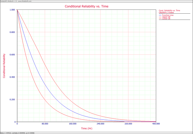
Weibull Disribution Conditional Reliability RRX Example
Median Rank Plot Example
In this example, we will determine the median rank value used for plotting the 6th failure from a sample size of 10. This example will use Weibull++'s Quick Statistical Reference (QSR) tool to show how the points in the plot of the following example are calculated.
First, open the Quick Statistical Reference tool and select the Inverse F-Distribution Values option.
In this example, n1 = 10, j = 6, m = 2(10 - 6 + 1) = 10, and n2 = 2 x 6 = 12.
Thus, from the F-distribution rank equation:
- [math]\displaystyle{ MR=\frac{1}{1+\left( \frac{10-6+1}{6} \right){{F}_{0.5;10;12}}}\,\! }[/math]
Use the QSR to calculate the value of F0.5;10;12 = 0.9886, as shown next:
Consequently:
- [math]\displaystyle{ MR=\frac{1}{1+\left( \frac{5}{6} \right)\times 0.9886}=0.5483=54.83%\,\! }[/math]
Another method is to use the Median Ranks option directly, which yields MR(%) = 54.8305%, as shown next:
Complete Data Example
Assume that 10 identical units (N = 10) are being reliability tested at the same application and operation stress levels. 6 of these units fail during this test after operating the following numbers of hours, [math]\displaystyle{ {T}_{j}\,\! }[/math]: 150, 105, 83, 123, 64 and 46. The test is stopped at the 6th failure. Find the parameters of the Weibull pdf that represents these data.
Solution
Create a new Weibull++ standard folio that is configured for grouped times-to-failure data with suspensions.
Enter the data in the appropriate columns. Note that there are 4 suspensions, as only 6 of the 10 units were tested to failure (the next figure shows the data as entered). Use the 3-parameter Weibull and MLE for the calculations.
Plot the data.
Note that the original data points, on the curved line, were adjusted by subtracting 30.92 hours to yield a straight line as shown above.
Suspension Data Example
ACME company manufactures widgets, and it is currently engaged in reliability testing a new widget design. 19 units are being reliability tested, but due to the tremendous demand for widgets, units are removed from the test whenever the production cannot cover the demand. The test is terminated at the 67th day when the last widget is removed from the test. The following table contains the collected data.
| Data Point Index | State (F/S) | Time to Failure |
| 1 | F | 2 |
| 2 | S | 3 |
| 3 | F | 5 |
| 4 | S | 7 |
| 5 | F | 11 |
| 6 | S | 13 |
| 7 | S | 17 |
| 8 | S | 19 |
| 9 | F | 23 |
| 10 | F | 29 |
| 11 | S | 31 |
| 12 | F | 37 |
| 13 | S | 41 |
| 14 | F | 43 |
| 15 | S | 47 |
| 16 | S | 53 |
| 17 | F | 59 |
| 18 | S | 61 |
| 19 | S | 67 |
Solution
In this example, we see that the number of failures is less than the number of suspensions. This is a very common situation, since reliability tests are often terminated before all units fail due to financial or time constraints. Furthermore, some suspensions will be recorded when a failure occurs that is not due to a legitimate failure mode, such as operator error. In cases such as this, a suspension is recorded, since the unit under test cannot be said to have had a legitimate failure.
Enter the data into a Weibull++ standard folio that is configured for times-to-failure data with suspensions. The folio will appear as shown next:
We will use the 2-parameter Weibull to solve this problem. The parameters using maximum likelihood are:
- [math]\displaystyle{ \begin{align} & \hat{\beta }=1.145 \\ & \hat{\eta }=65.97 \\ \end{align}\,\! }[/math]
Using RRX:
- [math]\displaystyle{ \begin{align} & \hat{\beta }=0.914\\ & \hat{\eta }=79.38 \\ \end{align}\,\! }[/math]
Using RRY:
- [math]\displaystyle{ \begin{align} & \hat{\beta }=0.895\\ & \hat{\eta }=82.02 \\ \end{align}\,\! }[/math]
Interval Data Example
Suppose we have run an experiment with 8 units tested and the following is a table of their last inspection times and failure times:
| Data Point Index | Last Inspection | Failure Time |
| 1 | 30 | 32 |
| 2 | 32 | 35 |
| 3 | 35 | 37 |
| 4 | 37 | 40 |
| 5 | 42 | 42 |
| 6 | 45 | 45 |
| 7 | 50 | 50 |
| 8 | 55 | 55 |
Analyze the data using several different parameter estimation techniques and compare the results.
Solution
Enter the data into a Weibull++ standard folio that is configured for interval data. The data is entered as follows:
The computed parameters using maximum likelihood are:
- [math]\displaystyle{ \begin{align} & \hat{\beta }=5.76 \\ & \hat{\eta }=44.68 \\ \end{align}\,\! }[/math]
Using RRX or rank regression on X:
- [math]\displaystyle{ \begin{align} & \hat{\beta }=5.70 \\ & \hat{\eta }=44.54 \\ \end{align}\,\! }[/math]
Using RRY or rank regression on Y:
- [math]\displaystyle{ \begin{align} & \hat{\beta }=5.41 \\ & \hat{\eta }=44.76 \\ \end{align}\,\! }[/math]
The plot of the MLE solution with the two-sided 90% confidence bounds is:
Mixed Data Types Example
From Dimitri Kececioglu, Reliability & Life Testing Handbook, Page 406. [20].
Estimate the parameters for the 3-parameter Weibull, for a sample of 10 units that are all tested to failure. The recorded failure times are 200; 370; 500; 620; 730; 840; 950; 1,050; 1,160 and 1,400 hours.
Published Results:
Published results (using probability plotting):
- [math]\displaystyle{ {\widehat{\beta}} = 3.0\,\! }[/math], [math]\displaystyle{ {\widehat{\eta}} = 1,220\,\! }[/math], [math]\displaystyle{ {\widehat{\gamma}} = -300\,\! }[/math]
Computed Results in Weibull++
Weibull++ computed parameters for rank regression on X are:
- [math]\displaystyle{ {\widehat{\beta}} = 2.9013\,\! }[/math], [math]\displaystyle{ {\widehat{\eta}} = 1195.5009\,\! }[/math], [math]\displaystyle{ {\widehat{\gamma}} = -279.000\,\! }[/math]
The small difference between the published results and the ones obtained from Weibull++ are due to the difference in the estimation method. In the publication the parameters were estimated using probability plotting (i.e., the fitted line was "eye-balled"). In Weibull++, the parameters were estimated using non-linear regression (a more accurate, mathematically fitted line). Note that γ in this example is negative. This means that the unadjusted for γ line is concave up, as shown next.
Weibull Distribution RRX Example
Assume that 6 identical units are being tested. The failure times are: 93, 34, 16, 120, 53 and 75 hours.
1. What is the unreliability of the units for a mission duration of 30 hours, starting the mission at age zero?
2. What is the reliability for a mission duration of 10 hours, starting the new mission at the age of T = 30 hours?
3. What is the longest mission that this product should undertake for a reliability of 90%?
Solution
1. First, we use Weibull++ to obtain the parameters using RRX.
Then, we investigate several methods of solution for this problem. The first, and more laborious, method is to extract the information directly from the plot. You may do this with either the screen plot in RS Draw or the printed copy of the plot. (When extracting information from the screen plot in RS Draw, note that the translated axis position of your mouse is always shown on the bottom right corner.)
Using this first method, enter either the screen plot or the printed plot with T = 30 hours, go up vertically to the straight line fitted to the data, then go horizontally to the ordinate, and read off the result. A good estimate of the unreliability is 23%. (Also, the reliability estimate is 1.0 - 0.23 = 0.77 or 77%.)
The second method involves the use of the Quick Calculation Pad (QCP).
Select the Prob. of Failure calculation option and enter 30 hours in the Mission End Time field.
Note that the results in QCP vary according to the parameter estimation method used. The above results are obtained using RRX.
2. The conditional reliability is given by:
- [math]\displaystyle{ R(t|T)=\frac{R(T+t)}{R(T)}\,\! }[/math]
or:
- [math]\displaystyle{ \hat{R}(10hr|30hr)=\frac{\hat{R}(10+30)}{\hat{R}(30)}=\frac{\hat{R}(40)}{\hat{R}(30)}\,\! }[/math]
Again, the QCP can provide this result directly and more accurately than the plot.
3. To use the QCP to solve for the longest mission that this product should undertake for a reliability of 90%, choose Reliable Life and enter 0.9 for the required reliability. The result is 15.9933 hours.
Benchmark with Published Examples
The following examples compare published results to computed results obtained with Weibull++.
Complete Data RRY Example
From Dimitri Kececioglu, Reliability & Life Testing Handbook, Page 418 [20].
Sample of 10 units, all tested to failure. The failures were recorded at 16, 34, 53, 75, 93, 120, 150, 191, 240 and 339 hours.
Published Results
Published Results (using Rank Regression on Y):
- [math]\displaystyle{ \begin{align} & \widehat{\beta }=1.20 \\ & \widehat{\eta} = 146.2 \\ & \hat{\rho }=0.998703\\ \end{align}\,\! }[/math]
Computed Results in Weibull++
This same data set can be entered into a Weibull++ standard data sheet. Use RRY for the estimation method.
Weibull++ computed parameters for RRY are:
- [math]\displaystyle{ \begin{align} & \widehat{\beta }=1.1973 \\ & \widehat{\eta} = 146.2545 \\ & \hat{\rho }=0.9999\\ \end{align}\,\! }[/math]
The small difference between the published results and the ones obtained from Weibull++ is due to the difference in the median rank values between the two (in the publication, median ranks are obtained from tables to 3 decimal places, whereas in Weibull++ they are calculated and carried out up to the 15th decimal point).
You will also notice that in the examples that follow, a small difference may exist between the published results and the ones obtained from Weibull++. This can be attributed to the difference between the computer numerical precision employed by Weibull++ and the lower number of significant digits used by the original authors. In most of these publications, no information was given as to the numerical precision used.
Suspension Data MLE Example
From Wayne Nelson, Fan Example, Applied Life Data Analysis, page 317 [30].
70 diesel engine fans accumulated 344,440 hours in service and 12 of them failed. A table of their life data is shown next (+ denotes non-failed units or suspensions, using Dr. Nelson's nomenclature). Evaluate the parameters with their two-sided 95% confidence bounds, using MLE for the 2-parameter Weibull distribution.
Published Results:
Weibull parameters (2P-Weibull, MLE):
- [math]\displaystyle{ \begin{align} & \widehat{\beta }=1.0584 \\ & \widehat{\eta} = 26,296 \\ \end{align}\,\! }[/math]
Published 95% FM confidence limits on the parameters:
- [math]\displaystyle{ \begin{align} & \widehat{\beta }=\lbrace 0.6441, \text{ }1.7394\rbrace \\ & \widehat{\eta} = \lbrace 10,522, \text{ }65,532\rbrace \\ \end{align}\,\! }[/math]
Published variance/covariance matrix:
Note that Nelson expresses the results as multiples of 1,000 (or = 26.297, etc.). The published results were adjusted by this factor to correlate with Weibull++ results.
Computed Results in Weibull++
This same data set can be entered into a Weibull++ standard folio, using 2-parameter Weibull and MLE to calculate the parameter estimates.
You can also enter the data as given in table without grouping them by opening a data sheet configured for suspension data. Then click the Group Data icon and chose Group exactly identical values.
The data will be automatically grouped and put into a new grouped data sheet.
Weibull++ computed parameters for maximum likelihood are:
- [math]\displaystyle{ \begin{align} & \widehat{\beta }=1.0584 \\ & \widehat{\eta} = 26,297 \\ \end{align}\,\! }[/math]
Weibull++ computed 95% FM confidence limits on the parameters:
- [math]\displaystyle{ \begin{align} & \widehat{\beta }=\lbrace 0.6441, \text{ }1.7394\rbrace \\ & \widehat{\eta} = \lbrace 10,522, \text{ }65,532\rbrace \\ \end{align}\,\! }[/math]
Weibull++ computed/variance covariance matrix:
The two-sided 95% bounds on the parameters can be determined from the QCP. Calculate and then click Report to see the results.
Interval Data MLE Example
From Wayne Nelson, Applied Life Data Analysis, Page 415 [30]. 167 identical parts were inspected for cracks. The following is a table of their last inspection times and times-to-failure:
Published Results:
Published results (using MLE):
- [math]\displaystyle{ \begin{align} & \widehat{\beta }=1.486 \\ & \widehat{\eta} = 71.687\\ \end{align}\,\! }[/math]
Published 95% FM confidence limits on the parameters:
- [math]\displaystyle{ \begin{align} & \widehat{\beta }=\lbrace 1.224, \text{ }1.802\rbrace \\ & \widehat{\eta} = \lbrace 61.962, \text{ }82.938\rbrace \\ \end{align}\,\! }[/math]
Published variance/covariance matrix:
Computed Results in Weibull++
This same data set can be entered into a Weibull++ standard folio that's configured for grouped times-to-failure data with suspensions and interval data.
Weibull++ computed parameters for maximum likelihood are:
- [math]\displaystyle{ \begin{align} & \widehat{\beta }=1.485 \\ & \widehat{\eta} = 71.690\\ \end{align}\,\! }[/math]
Weibull++ computed 95% FM confidence limits on the parameters:
- [math]\displaystyle{ \begin{align} & \widehat{\beta }=\lbrace 1.224, \text{ }1.802\rbrace \\ & \widehat{\eta} = \lbrace 61.961, \text{ }82.947\rbrace \\ \end{align}\,\! }[/math]
Weibull++ computed/variance covariance matrix:
Grouped Suspension MLE Example
From Dallas R. Wingo, IEEE Transactions on Reliability Vol. R-22, No 2, June 1973, Pages 96-100.
Wingo uses the following times-to-failure: 37, 55, 64, 72, 74, 87, 88, 89, 91, 92, 94, 95, 97, 98, 100, 101, 102, 102, 105, 105, 107, 113, 117, 120, 120, 120, 122, 124, 126, 130, 135, 138, 182. In addition, the following suspensions are used: 4 at 70, 5 at 80, 4 at 99, 3 at 121 and 1 at 150.
Published Results (using MLE)
- [math]\displaystyle{ \begin{align} & \widehat{\beta }=3.7596935\\ & \widehat{\eta} = 106.49758 \\ & \hat{\gamma }=14.451684\\ \end{align}\,\! }[/math]
Computed Results in Weibull++
- [math]\displaystyle{ \begin{align} & \widehat{\beta }=3.7596935\\ & \widehat{\eta} = 106.49758 \\ & \hat{\gamma }=14.451684\\ \end{align}\,\! }[/math]
Note that you must select the Use True 3-P MLEoption in the Weibull++ Application Setup to replicate these results.
3-P Probability Plot Example
Suppose we want to model a left censored, right censored, interval, and complete data set, consisting of 274 units under test of which 185 units fail. The following table contains the data.
| Data Point Index | Number in State | Last Inspection | State (S or F) | State End Time |
| 1 | 2 | 5 | F | 5 |
| 2 | 23 | 5 | S | 5 |
| 3 | 28 | 0 | F | 7 |
| 4 | 4 | 10 | F | 10 |
| 5 | 7 | 15 | F | 15 |
| 6 | 8 | 20 | F | 20 |
| 7 | 29 | 20 | S | 20 |
| 8 | 32 | 0 | F | 22 |
| 9 | 6 | 25 | F | 25 |
| 10 | 4 | 27 | F | 30 |
| 11 | 8 | 30 | F | 35 |
| 12 | 5 | 30 | F | 40 |
| 13 | 9 | 27 | F | 45 |
| 14 | 7 | 25 | F | 50 |
| 15 | 5 | 20 | F | 55 |
| 16 | 3 | 15 | F | 60 |
| 17 | 6 | 10 | F | 65 |
| 18 | 3 | 5 | F | 70 |
| 19 | 37 | 100 | S | 100 |
| 20 | 48 | 0 | F | 102 |
Solution
Since standard ranking methods for dealing with these different data types are inadequate, we will want to use the ReliaSoft ranking method. This option is the default in Weibull++ when dealing with interval data. The filled-out standard folio is shown next:
The computed parameters using MLE are:
- [math]\displaystyle{ \hat{\beta }=0.748;\text{ }\hat{\eta }=44.38\,\! }[/math]
Using RRX:
- [math]\displaystyle{ \hat{\beta }=1.057;\text{ }\hat{\eta }=36.29\,\! }[/math]
Using RRY:
- [math]\displaystyle{ \hat{\beta }=0.998;\text{ }\hat{\eta }=37.16\,\! }[/math]
The plot with the two-sided 90% confidence bounds for the rank regression on X solution is:
Weibull Distribution Reliable Life RRX Example
Median Rank Plot Example
In this example, we will determine the median rank value used for plotting the 6th failure from a sample size of 10. This example will use Weibull++'s Quick Statistical Reference (QSR) tool to show how the points in the plot of the following example are calculated.
First, open the Quick Statistical Reference tool and select the Inverse F-Distribution Values option.
In this example, n1 = 10, j = 6, m = 2(10 - 6 + 1) = 10, and n2 = 2 x 6 = 12.
Thus, from the F-distribution rank equation:
- [math]\displaystyle{ MR=\frac{1}{1+\left( \frac{10-6+1}{6} \right){{F}_{0.5;10;12}}}\,\! }[/math]
Use the QSR to calculate the value of F0.5;10;12 = 0.9886, as shown next:
Consequently:
- [math]\displaystyle{ MR=\frac{1}{1+\left( \frac{5}{6} \right)\times 0.9886}=0.5483=54.83%\,\! }[/math]
Another method is to use the Median Ranks option directly, which yields MR(%) = 54.8305%, as shown next:
Complete Data Example
Assume that 10 identical units (N = 10) are being reliability tested at the same application and operation stress levels. 6 of these units fail during this test after operating the following numbers of hours, [math]\displaystyle{ {T}_{j}\,\! }[/math]: 150, 105, 83, 123, 64 and 46. The test is stopped at the 6th failure. Find the parameters of the Weibull pdf that represents these data.
Solution
Create a new Weibull++ standard folio that is configured for grouped times-to-failure data with suspensions.
Enter the data in the appropriate columns. Note that there are 4 suspensions, as only 6 of the 10 units were tested to failure (the next figure shows the data as entered). Use the 3-parameter Weibull and MLE for the calculations.
Plot the data.
Note that the original data points, on the curved line, were adjusted by subtracting 30.92 hours to yield a straight line as shown above.
Suspension Data Example
ACME company manufactures widgets, and it is currently engaged in reliability testing a new widget design. 19 units are being reliability tested, but due to the tremendous demand for widgets, units are removed from the test whenever the production cannot cover the demand. The test is terminated at the 67th day when the last widget is removed from the test. The following table contains the collected data.
| Data Point Index | State (F/S) | Time to Failure |
| 1 | F | 2 |
| 2 | S | 3 |
| 3 | F | 5 |
| 4 | S | 7 |
| 5 | F | 11 |
| 6 | S | 13 |
| 7 | S | 17 |
| 8 | S | 19 |
| 9 | F | 23 |
| 10 | F | 29 |
| 11 | S | 31 |
| 12 | F | 37 |
| 13 | S | 41 |
| 14 | F | 43 |
| 15 | S | 47 |
| 16 | S | 53 |
| 17 | F | 59 |
| 18 | S | 61 |
| 19 | S | 67 |
Solution
In this example, we see that the number of failures is less than the number of suspensions. This is a very common situation, since reliability tests are often terminated before all units fail due to financial or time constraints. Furthermore, some suspensions will be recorded when a failure occurs that is not due to a legitimate failure mode, such as operator error. In cases such as this, a suspension is recorded, since the unit under test cannot be said to have had a legitimate failure.
Enter the data into a Weibull++ standard folio that is configured for times-to-failure data with suspensions. The folio will appear as shown next:
We will use the 2-parameter Weibull to solve this problem. The parameters using maximum likelihood are:
- [math]\displaystyle{ \begin{align} & \hat{\beta }=1.145 \\ & \hat{\eta }=65.97 \\ \end{align}\,\! }[/math]
Using RRX:
- [math]\displaystyle{ \begin{align} & \hat{\beta }=0.914\\ & \hat{\eta }=79.38 \\ \end{align}\,\! }[/math]
Using RRY:
- [math]\displaystyle{ \begin{align} & \hat{\beta }=0.895\\ & \hat{\eta }=82.02 \\ \end{align}\,\! }[/math]
Interval Data Example
Suppose we have run an experiment with 8 units tested and the following is a table of their last inspection times and failure times:
| Data Point Index | Last Inspection | Failure Time |
| 1 | 30 | 32 |
| 2 | 32 | 35 |
| 3 | 35 | 37 |
| 4 | 37 | 40 |
| 5 | 42 | 42 |
| 6 | 45 | 45 |
| 7 | 50 | 50 |
| 8 | 55 | 55 |
Analyze the data using several different parameter estimation techniques and compare the results.
Solution
Enter the data into a Weibull++ standard folio that is configured for interval data. The data is entered as follows:
The computed parameters using maximum likelihood are:
- [math]\displaystyle{ \begin{align} & \hat{\beta }=5.76 \\ & \hat{\eta }=44.68 \\ \end{align}\,\! }[/math]
Using RRX or rank regression on X:
- [math]\displaystyle{ \begin{align} & \hat{\beta }=5.70 \\ & \hat{\eta }=44.54 \\ \end{align}\,\! }[/math]
Using RRY or rank regression on Y:
- [math]\displaystyle{ \begin{align} & \hat{\beta }=5.41 \\ & \hat{\eta }=44.76 \\ \end{align}\,\! }[/math]
The plot of the MLE solution with the two-sided 90% confidence bounds is:
Mixed Data Types Example
From Dimitri Kececioglu, Reliability & Life Testing Handbook, Page 406. [20].
Estimate the parameters for the 3-parameter Weibull, for a sample of 10 units that are all tested to failure. The recorded failure times are 200; 370; 500; 620; 730; 840; 950; 1,050; 1,160 and 1,400 hours.
Published Results:
Published results (using probability plotting):
- [math]\displaystyle{ {\widehat{\beta}} = 3.0\,\! }[/math], [math]\displaystyle{ {\widehat{\eta}} = 1,220\,\! }[/math], [math]\displaystyle{ {\widehat{\gamma}} = -300\,\! }[/math]
Computed Results in Weibull++
Weibull++ computed parameters for rank regression on X are:
- [math]\displaystyle{ {\widehat{\beta}} = 2.9013\,\! }[/math], [math]\displaystyle{ {\widehat{\eta}} = 1195.5009\,\! }[/math], [math]\displaystyle{ {\widehat{\gamma}} = -279.000\,\! }[/math]
The small difference between the published results and the ones obtained from Weibull++ are due to the difference in the estimation method. In the publication the parameters were estimated using probability plotting (i.e., the fitted line was "eye-balled"). In Weibull++, the parameters were estimated using non-linear regression (a more accurate, mathematically fitted line). Note that γ in this example is negative. This means that the unadjusted for γ line is concave up, as shown next.
Weibull Distribution RRX Example
Assume that 6 identical units are being tested. The failure times are: 93, 34, 16, 120, 53 and 75 hours.
1. What is the unreliability of the units for a mission duration of 30 hours, starting the mission at age zero?
2. What is the reliability for a mission duration of 10 hours, starting the new mission at the age of T = 30 hours?
3. What is the longest mission that this product should undertake for a reliability of 90%?
Solution
1. First, we use Weibull++ to obtain the parameters using RRX.
Then, we investigate several methods of solution for this problem. The first, and more laborious, method is to extract the information directly from the plot. You may do this with either the screen plot in RS Draw or the printed copy of the plot. (When extracting information from the screen plot in RS Draw, note that the translated axis position of your mouse is always shown on the bottom right corner.)
Using this first method, enter either the screen plot or the printed plot with T = 30 hours, go up vertically to the straight line fitted to the data, then go horizontally to the ordinate, and read off the result. A good estimate of the unreliability is 23%. (Also, the reliability estimate is 1.0 - 0.23 = 0.77 or 77%.)
The second method involves the use of the Quick Calculation Pad (QCP).
Select the Prob. of Failure calculation option and enter 30 hours in the Mission End Time field.
Note that the results in QCP vary according to the parameter estimation method used. The above results are obtained using RRX.
2. The conditional reliability is given by:
- [math]\displaystyle{ R(t|T)=\frac{R(T+t)}{R(T)}\,\! }[/math]
or:
- [math]\displaystyle{ \hat{R}(10hr|30hr)=\frac{\hat{R}(10+30)}{\hat{R}(30)}=\frac{\hat{R}(40)}{\hat{R}(30)}\,\! }[/math]
Again, the QCP can provide this result directly and more accurately than the plot.
3. To use the QCP to solve for the longest mission that this product should undertake for a reliability of 90%, choose Reliable Life and enter 0.9 for the required reliability. The result is 15.9933 hours.
Benchmark with Published Examples
The following examples compare published results to computed results obtained with Weibull++.
Complete Data RRY Example
From Dimitri Kececioglu, Reliability & Life Testing Handbook, Page 418 [20].
Sample of 10 units, all tested to failure. The failures were recorded at 16, 34, 53, 75, 93, 120, 150, 191, 240 and 339 hours.
Published Results
Published Results (using Rank Regression on Y):
- [math]\displaystyle{ \begin{align} & \widehat{\beta }=1.20 \\ & \widehat{\eta} = 146.2 \\ & \hat{\rho }=0.998703\\ \end{align}\,\! }[/math]
Computed Results in Weibull++
This same data set can be entered into a Weibull++ standard data sheet. Use RRY for the estimation method.
Weibull++ computed parameters for RRY are:
- [math]\displaystyle{ \begin{align} & \widehat{\beta }=1.1973 \\ & \widehat{\eta} = 146.2545 \\ & \hat{\rho }=0.9999\\ \end{align}\,\! }[/math]
The small difference between the published results and the ones obtained from Weibull++ is due to the difference in the median rank values between the two (in the publication, median ranks are obtained from tables to 3 decimal places, whereas in Weibull++ they are calculated and carried out up to the 15th decimal point).
You will also notice that in the examples that follow, a small difference may exist between the published results and the ones obtained from Weibull++. This can be attributed to the difference between the computer numerical precision employed by Weibull++ and the lower number of significant digits used by the original authors. In most of these publications, no information was given as to the numerical precision used.
Suspension Data MLE Example
From Wayne Nelson, Fan Example, Applied Life Data Analysis, page 317 [30].
70 diesel engine fans accumulated 344,440 hours in service and 12 of them failed. A table of their life data is shown next (+ denotes non-failed units or suspensions, using Dr. Nelson's nomenclature). Evaluate the parameters with their two-sided 95% confidence bounds, using MLE for the 2-parameter Weibull distribution.
Published Results:
Weibull parameters (2P-Weibull, MLE):
- [math]\displaystyle{ \begin{align} & \widehat{\beta }=1.0584 \\ & \widehat{\eta} = 26,296 \\ \end{align}\,\! }[/math]
Published 95% FM confidence limits on the parameters:
- [math]\displaystyle{ \begin{align} & \widehat{\beta }=\lbrace 0.6441, \text{ }1.7394\rbrace \\ & \widehat{\eta} = \lbrace 10,522, \text{ }65,532\rbrace \\ \end{align}\,\! }[/math]
Published variance/covariance matrix:
Note that Nelson expresses the results as multiples of 1,000 (or = 26.297, etc.). The published results were adjusted by this factor to correlate with Weibull++ results.
Computed Results in Weibull++
This same data set can be entered into a Weibull++ standard folio, using 2-parameter Weibull and MLE to calculate the parameter estimates.
You can also enter the data as given in table without grouping them by opening a data sheet configured for suspension data. Then click the Group Data icon and chose Group exactly identical values.
The data will be automatically grouped and put into a new grouped data sheet.
Weibull++ computed parameters for maximum likelihood are:
- [math]\displaystyle{ \begin{align} & \widehat{\beta }=1.0584 \\ & \widehat{\eta} = 26,297 \\ \end{align}\,\! }[/math]
Weibull++ computed 95% FM confidence limits on the parameters:
- [math]\displaystyle{ \begin{align} & \widehat{\beta }=\lbrace 0.6441, \text{ }1.7394\rbrace \\ & \widehat{\eta} = \lbrace 10,522, \text{ }65,532\rbrace \\ \end{align}\,\! }[/math]
Weibull++ computed/variance covariance matrix:
The two-sided 95% bounds on the parameters can be determined from the QCP. Calculate and then click Report to see the results.
Interval Data MLE Example
From Wayne Nelson, Applied Life Data Analysis, Page 415 [30]. 167 identical parts were inspected for cracks. The following is a table of their last inspection times and times-to-failure:
Published Results:
Published results (using MLE):
- [math]\displaystyle{ \begin{align} & \widehat{\beta }=1.486 \\ & \widehat{\eta} = 71.687\\ \end{align}\,\! }[/math]
Published 95% FM confidence limits on the parameters:
- [math]\displaystyle{ \begin{align} & \widehat{\beta }=\lbrace 1.224, \text{ }1.802\rbrace \\ & \widehat{\eta} = \lbrace 61.962, \text{ }82.938\rbrace \\ \end{align}\,\! }[/math]
Published variance/covariance matrix:
Computed Results in Weibull++
This same data set can be entered into a Weibull++ standard folio that's configured for grouped times-to-failure data with suspensions and interval data.
Weibull++ computed parameters for maximum likelihood are:
- [math]\displaystyle{ \begin{align} & \widehat{\beta }=1.485 \\ & \widehat{\eta} = 71.690\\ \end{align}\,\! }[/math]
Weibull++ computed 95% FM confidence limits on the parameters:
- [math]\displaystyle{ \begin{align} & \widehat{\beta }=\lbrace 1.224, \text{ }1.802\rbrace \\ & \widehat{\eta} = \lbrace 61.961, \text{ }82.947\rbrace \\ \end{align}\,\! }[/math]
Weibull++ computed/variance covariance matrix:
Grouped Suspension MLE Example
From Dallas R. Wingo, IEEE Transactions on Reliability Vol. R-22, No 2, June 1973, Pages 96-100.
Wingo uses the following times-to-failure: 37, 55, 64, 72, 74, 87, 88, 89, 91, 92, 94, 95, 97, 98, 100, 101, 102, 102, 105, 105, 107, 113, 117, 120, 120, 120, 122, 124, 126, 130, 135, 138, 182. In addition, the following suspensions are used: 4 at 70, 5 at 80, 4 at 99, 3 at 121 and 1 at 150.
Published Results (using MLE)
- [math]\displaystyle{ \begin{align} & \widehat{\beta }=3.7596935\\ & \widehat{\eta} = 106.49758 \\ & \hat{\gamma }=14.451684\\ \end{align}\,\! }[/math]
Computed Results in Weibull++
- [math]\displaystyle{ \begin{align} & \widehat{\beta }=3.7596935\\ & \widehat{\eta} = 106.49758 \\ & \hat{\gamma }=14.451684\\ \end{align}\,\! }[/math]
Note that you must select the Use True 3-P MLEoption in the Weibull++ Application Setup to replicate these results.
3-P Probability Plot Example
Suppose we want to model a left censored, right censored, interval, and complete data set, consisting of 274 units under test of which 185 units fail. The following table contains the data.
| Data Point Index | Number in State | Last Inspection | State (S or F) | State End Time |
| 1 | 2 | 5 | F | 5 |
| 2 | 23 | 5 | S | 5 |
| 3 | 28 | 0 | F | 7 |
| 4 | 4 | 10 | F | 10 |
| 5 | 7 | 15 | F | 15 |
| 6 | 8 | 20 | F | 20 |
| 7 | 29 | 20 | S | 20 |
| 8 | 32 | 0 | F | 22 |
| 9 | 6 | 25 | F | 25 |
| 10 | 4 | 27 | F | 30 |
| 11 | 8 | 30 | F | 35 |
| 12 | 5 | 30 | F | 40 |
| 13 | 9 | 27 | F | 45 |
| 14 | 7 | 25 | F | 50 |
| 15 | 5 | 20 | F | 55 |
| 16 | 3 | 15 | F | 60 |
| 17 | 6 | 10 | F | 65 |
| 18 | 3 | 5 | F | 70 |
| 19 | 37 | 100 | S | 100 |
| 20 | 48 | 0 | F | 102 |
Solution
Since standard ranking methods for dealing with these different data types are inadequate, we will want to use the ReliaSoft ranking method. This option is the default in Weibull++ when dealing with interval data. The filled-out standard folio is shown next:
The computed parameters using MLE are:
- [math]\displaystyle{ \hat{\beta }=0.748;\text{ }\hat{\eta }=44.38\,\! }[/math]
Using RRX:
- [math]\displaystyle{ \hat{\beta }=1.057;\text{ }\hat{\eta }=36.29\,\! }[/math]
Using RRY:
- [math]\displaystyle{ \hat{\beta }=0.998;\text{ }\hat{\eta }=37.16\,\! }[/math]
The plot with the two-sided 90% confidence bounds for the rank regression on X solution is:
Weibull Distribution Complete Data Example
Median Rank Plot Example
In this example, we will determine the median rank value used for plotting the 6th failure from a sample size of 10. This example will use Weibull++'s Quick Statistical Reference (QSR) tool to show how the points in the plot of the following example are calculated.
First, open the Quick Statistical Reference tool and select the Inverse F-Distribution Values option.
In this example, n1 = 10, j = 6, m = 2(10 - 6 + 1) = 10, and n2 = 2 x 6 = 12.
Thus, from the F-distribution rank equation:
- [math]\displaystyle{ MR=\frac{1}{1+\left( \frac{10-6+1}{6} \right){{F}_{0.5;10;12}}}\,\! }[/math]
Use the QSR to calculate the value of F0.5;10;12 = 0.9886, as shown next:
Consequently:
- [math]\displaystyle{ MR=\frac{1}{1+\left( \frac{5}{6} \right)\times 0.9886}=0.5483=54.83%\,\! }[/math]
Another method is to use the Median Ranks option directly, which yields MR(%) = 54.8305%, as shown next:
Complete Data Example
Assume that 10 identical units (N = 10) are being reliability tested at the same application and operation stress levels. 6 of these units fail during this test after operating the following numbers of hours, [math]\displaystyle{ {T}_{j}\,\! }[/math]: 150, 105, 83, 123, 64 and 46. The test is stopped at the 6th failure. Find the parameters of the Weibull pdf that represents these data.
Solution
Create a new Weibull++ standard folio that is configured for grouped times-to-failure data with suspensions.
Enter the data in the appropriate columns. Note that there are 4 suspensions, as only 6 of the 10 units were tested to failure (the next figure shows the data as entered). Use the 3-parameter Weibull and MLE for the calculations.
Plot the data.
Note that the original data points, on the curved line, were adjusted by subtracting 30.92 hours to yield a straight line as shown above.
Suspension Data Example
ACME company manufactures widgets, and it is currently engaged in reliability testing a new widget design. 19 units are being reliability tested, but due to the tremendous demand for widgets, units are removed from the test whenever the production cannot cover the demand. The test is terminated at the 67th day when the last widget is removed from the test. The following table contains the collected data.
| Data Point Index | State (F/S) | Time to Failure |
| 1 | F | 2 |
| 2 | S | 3 |
| 3 | F | 5 |
| 4 | S | 7 |
| 5 | F | 11 |
| 6 | S | 13 |
| 7 | S | 17 |
| 8 | S | 19 |
| 9 | F | 23 |
| 10 | F | 29 |
| 11 | S | 31 |
| 12 | F | 37 |
| 13 | S | 41 |
| 14 | F | 43 |
| 15 | S | 47 |
| 16 | S | 53 |
| 17 | F | 59 |
| 18 | S | 61 |
| 19 | S | 67 |
Solution
In this example, we see that the number of failures is less than the number of suspensions. This is a very common situation, since reliability tests are often terminated before all units fail due to financial or time constraints. Furthermore, some suspensions will be recorded when a failure occurs that is not due to a legitimate failure mode, such as operator error. In cases such as this, a suspension is recorded, since the unit under test cannot be said to have had a legitimate failure.
Enter the data into a Weibull++ standard folio that is configured for times-to-failure data with suspensions. The folio will appear as shown next:
We will use the 2-parameter Weibull to solve this problem. The parameters using maximum likelihood are:
- [math]\displaystyle{ \begin{align} & \hat{\beta }=1.145 \\ & \hat{\eta }=65.97 \\ \end{align}\,\! }[/math]
Using RRX:
- [math]\displaystyle{ \begin{align} & \hat{\beta }=0.914\\ & \hat{\eta }=79.38 \\ \end{align}\,\! }[/math]
Using RRY:
- [math]\displaystyle{ \begin{align} & \hat{\beta }=0.895\\ & \hat{\eta }=82.02 \\ \end{align}\,\! }[/math]
Interval Data Example
Suppose we have run an experiment with 8 units tested and the following is a table of their last inspection times and failure times:
| Data Point Index | Last Inspection | Failure Time |
| 1 | 30 | 32 |
| 2 | 32 | 35 |
| 3 | 35 | 37 |
| 4 | 37 | 40 |
| 5 | 42 | 42 |
| 6 | 45 | 45 |
| 7 | 50 | 50 |
| 8 | 55 | 55 |
Analyze the data using several different parameter estimation techniques and compare the results.
Solution
Enter the data into a Weibull++ standard folio that is configured for interval data. The data is entered as follows:
The computed parameters using maximum likelihood are:
- [math]\displaystyle{ \begin{align} & \hat{\beta }=5.76 \\ & \hat{\eta }=44.68 \\ \end{align}\,\! }[/math]
Using RRX or rank regression on X:
- [math]\displaystyle{ \begin{align} & \hat{\beta }=5.70 \\ & \hat{\eta }=44.54 \\ \end{align}\,\! }[/math]
Using RRY or rank regression on Y:
- [math]\displaystyle{ \begin{align} & \hat{\beta }=5.41 \\ & \hat{\eta }=44.76 \\ \end{align}\,\! }[/math]
The plot of the MLE solution with the two-sided 90% confidence bounds is:
Mixed Data Types Example
From Dimitri Kececioglu, Reliability & Life Testing Handbook, Page 406. [20].
Estimate the parameters for the 3-parameter Weibull, for a sample of 10 units that are all tested to failure. The recorded failure times are 200; 370; 500; 620; 730; 840; 950; 1,050; 1,160 and 1,400 hours.
Published Results:
Published results (using probability plotting):
- [math]\displaystyle{ {\widehat{\beta}} = 3.0\,\! }[/math], [math]\displaystyle{ {\widehat{\eta}} = 1,220\,\! }[/math], [math]\displaystyle{ {\widehat{\gamma}} = -300\,\! }[/math]
Computed Results in Weibull++
Weibull++ computed parameters for rank regression on X are:
- [math]\displaystyle{ {\widehat{\beta}} = 2.9013\,\! }[/math], [math]\displaystyle{ {\widehat{\eta}} = 1195.5009\,\! }[/math], [math]\displaystyle{ {\widehat{\gamma}} = -279.000\,\! }[/math]
The small difference between the published results and the ones obtained from Weibull++ are due to the difference in the estimation method. In the publication the parameters were estimated using probability plotting (i.e., the fitted line was "eye-balled"). In Weibull++, the parameters were estimated using non-linear regression (a more accurate, mathematically fitted line). Note that γ in this example is negative. This means that the unadjusted for γ line is concave up, as shown next.
Weibull Distribution RRX Example
Assume that 6 identical units are being tested. The failure times are: 93, 34, 16, 120, 53 and 75 hours.
1. What is the unreliability of the units for a mission duration of 30 hours, starting the mission at age zero?
2. What is the reliability for a mission duration of 10 hours, starting the new mission at the age of T = 30 hours?
3. What is the longest mission that this product should undertake for a reliability of 90%?
Solution
1. First, we use Weibull++ to obtain the parameters using RRX.
Then, we investigate several methods of solution for this problem. The first, and more laborious, method is to extract the information directly from the plot. You may do this with either the screen plot in RS Draw or the printed copy of the plot. (When extracting information from the screen plot in RS Draw, note that the translated axis position of your mouse is always shown on the bottom right corner.)
Using this first method, enter either the screen plot or the printed plot with T = 30 hours, go up vertically to the straight line fitted to the data, then go horizontally to the ordinate, and read off the result. A good estimate of the unreliability is 23%. (Also, the reliability estimate is 1.0 - 0.23 = 0.77 or 77%.)
The second method involves the use of the Quick Calculation Pad (QCP).
Select the Prob. of Failure calculation option and enter 30 hours in the Mission End Time field.
Note that the results in QCP vary according to the parameter estimation method used. The above results are obtained using RRX.
2. The conditional reliability is given by:
- [math]\displaystyle{ R(t|T)=\frac{R(T+t)}{R(T)}\,\! }[/math]
or:
- [math]\displaystyle{ \hat{R}(10hr|30hr)=\frac{\hat{R}(10+30)}{\hat{R}(30)}=\frac{\hat{R}(40)}{\hat{R}(30)}\,\! }[/math]
Again, the QCP can provide this result directly and more accurately than the plot.
3. To use the QCP to solve for the longest mission that this product should undertake for a reliability of 90%, choose Reliable Life and enter 0.9 for the required reliability. The result is 15.9933 hours.
Benchmark with Published Examples
The following examples compare published results to computed results obtained with Weibull++.
Complete Data RRY Example
From Dimitri Kececioglu, Reliability & Life Testing Handbook, Page 418 [20].
Sample of 10 units, all tested to failure. The failures were recorded at 16, 34, 53, 75, 93, 120, 150, 191, 240 and 339 hours.
Published Results
Published Results (using Rank Regression on Y):
- [math]\displaystyle{ \begin{align} & \widehat{\beta }=1.20 \\ & \widehat{\eta} = 146.2 \\ & \hat{\rho }=0.998703\\ \end{align}\,\! }[/math]
Computed Results in Weibull++
This same data set can be entered into a Weibull++ standard data sheet. Use RRY for the estimation method.
Weibull++ computed parameters for RRY are:
- [math]\displaystyle{ \begin{align} & \widehat{\beta }=1.1973 \\ & \widehat{\eta} = 146.2545 \\ & \hat{\rho }=0.9999\\ \end{align}\,\! }[/math]
The small difference between the published results and the ones obtained from Weibull++ is due to the difference in the median rank values between the two (in the publication, median ranks are obtained from tables to 3 decimal places, whereas in Weibull++ they are calculated and carried out up to the 15th decimal point).
You will also notice that in the examples that follow, a small difference may exist between the published results and the ones obtained from Weibull++. This can be attributed to the difference between the computer numerical precision employed by Weibull++ and the lower number of significant digits used by the original authors. In most of these publications, no information was given as to the numerical precision used.
Suspension Data MLE Example
From Wayne Nelson, Fan Example, Applied Life Data Analysis, page 317 [30].
70 diesel engine fans accumulated 344,440 hours in service and 12 of them failed. A table of their life data is shown next (+ denotes non-failed units or suspensions, using Dr. Nelson's nomenclature). Evaluate the parameters with their two-sided 95% confidence bounds, using MLE for the 2-parameter Weibull distribution.
Published Results:
Weibull parameters (2P-Weibull, MLE):
- [math]\displaystyle{ \begin{align} & \widehat{\beta }=1.0584 \\ & \widehat{\eta} = 26,296 \\ \end{align}\,\! }[/math]
Published 95% FM confidence limits on the parameters:
- [math]\displaystyle{ \begin{align} & \widehat{\beta }=\lbrace 0.6441, \text{ }1.7394\rbrace \\ & \widehat{\eta} = \lbrace 10,522, \text{ }65,532\rbrace \\ \end{align}\,\! }[/math]
Published variance/covariance matrix:
Note that Nelson expresses the results as multiples of 1,000 (or = 26.297, etc.). The published results were adjusted by this factor to correlate with Weibull++ results.
Computed Results in Weibull++
This same data set can be entered into a Weibull++ standard folio, using 2-parameter Weibull and MLE to calculate the parameter estimates.
You can also enter the data as given in table without grouping them by opening a data sheet configured for suspension data. Then click the Group Data icon and chose Group exactly identical values.
The data will be automatically grouped and put into a new grouped data sheet.
Weibull++ computed parameters for maximum likelihood are:
- [math]\displaystyle{ \begin{align} & \widehat{\beta }=1.0584 \\ & \widehat{\eta} = 26,297 \\ \end{align}\,\! }[/math]
Weibull++ computed 95% FM confidence limits on the parameters:
- [math]\displaystyle{ \begin{align} & \widehat{\beta }=\lbrace 0.6441, \text{ }1.7394\rbrace \\ & \widehat{\eta} = \lbrace 10,522, \text{ }65,532\rbrace \\ \end{align}\,\! }[/math]
Weibull++ computed/variance covariance matrix:
The two-sided 95% bounds on the parameters can be determined from the QCP. Calculate and then click Report to see the results.
Interval Data MLE Example
From Wayne Nelson, Applied Life Data Analysis, Page 415 [30]. 167 identical parts were inspected for cracks. The following is a table of their last inspection times and times-to-failure:
Published Results:
Published results (using MLE):
- [math]\displaystyle{ \begin{align} & \widehat{\beta }=1.486 \\ & \widehat{\eta} = 71.687\\ \end{align}\,\! }[/math]
Published 95% FM confidence limits on the parameters:
- [math]\displaystyle{ \begin{align} & \widehat{\beta }=\lbrace 1.224, \text{ }1.802\rbrace \\ & \widehat{\eta} = \lbrace 61.962, \text{ }82.938\rbrace \\ \end{align}\,\! }[/math]
Published variance/covariance matrix:
Computed Results in Weibull++
This same data set can be entered into a Weibull++ standard folio that's configured for grouped times-to-failure data with suspensions and interval data.
Weibull++ computed parameters for maximum likelihood are:
- [math]\displaystyle{ \begin{align} & \widehat{\beta }=1.485 \\ & \widehat{\eta} = 71.690\\ \end{align}\,\! }[/math]
Weibull++ computed 95% FM confidence limits on the parameters:
- [math]\displaystyle{ \begin{align} & \widehat{\beta }=\lbrace 1.224, \text{ }1.802\rbrace \\ & \widehat{\eta} = \lbrace 61.961, \text{ }82.947\rbrace \\ \end{align}\,\! }[/math]
Weibull++ computed/variance covariance matrix:
Grouped Suspension MLE Example
From Dallas R. Wingo, IEEE Transactions on Reliability Vol. R-22, No 2, June 1973, Pages 96-100.
Wingo uses the following times-to-failure: 37, 55, 64, 72, 74, 87, 88, 89, 91, 92, 94, 95, 97, 98, 100, 101, 102, 102, 105, 105, 107, 113, 117, 120, 120, 120, 122, 124, 126, 130, 135, 138, 182. In addition, the following suspensions are used: 4 at 70, 5 at 80, 4 at 99, 3 at 121 and 1 at 150.
Published Results (using MLE)
- [math]\displaystyle{ \begin{align} & \widehat{\beta }=3.7596935\\ & \widehat{\eta} = 106.49758 \\ & \hat{\gamma }=14.451684\\ \end{align}\,\! }[/math]
Computed Results in Weibull++
- [math]\displaystyle{ \begin{align} & \widehat{\beta }=3.7596935\\ & \widehat{\eta} = 106.49758 \\ & \hat{\gamma }=14.451684\\ \end{align}\,\! }[/math]
Note that you must select the Use True 3-P MLEoption in the Weibull++ Application Setup to replicate these results.
3-P Probability Plot Example
Suppose we want to model a left censored, right censored, interval, and complete data set, consisting of 274 units under test of which 185 units fail. The following table contains the data.
| Data Point Index | Number in State | Last Inspection | State (S or F) | State End Time |
| 1 | 2 | 5 | F | 5 |
| 2 | 23 | 5 | S | 5 |
| 3 | 28 | 0 | F | 7 |
| 4 | 4 | 10 | F | 10 |
| 5 | 7 | 15 | F | 15 |
| 6 | 8 | 20 | F | 20 |
| 7 | 29 | 20 | S | 20 |
| 8 | 32 | 0 | F | 22 |
| 9 | 6 | 25 | F | 25 |
| 10 | 4 | 27 | F | 30 |
| 11 | 8 | 30 | F | 35 |
| 12 | 5 | 30 | F | 40 |
| 13 | 9 | 27 | F | 45 |
| 14 | 7 | 25 | F | 50 |
| 15 | 5 | 20 | F | 55 |
| 16 | 3 | 15 | F | 60 |
| 17 | 6 | 10 | F | 65 |
| 18 | 3 | 5 | F | 70 |
| 19 | 37 | 100 | S | 100 |
| 20 | 48 | 0 | F | 102 |
Solution
Since standard ranking methods for dealing with these different data types are inadequate, we will want to use the ReliaSoft ranking method. This option is the default in Weibull++ when dealing with interval data. The filled-out standard folio is shown next:
The computed parameters using MLE are:
- [math]\displaystyle{ \hat{\beta }=0.748;\text{ }\hat{\eta }=44.38\,\! }[/math]
Using RRX:
- [math]\displaystyle{ \hat{\beta }=1.057;\text{ }\hat{\eta }=36.29\,\! }[/math]
Using RRY:
- [math]\displaystyle{ \hat{\beta }=0.998;\text{ }\hat{\eta }=37.16\,\! }[/math]
The plot with the two-sided 90% confidence bounds for the rank regression on X solution is:
Weibull Distribution Interval Data Example
Median Rank Plot Example
In this example, we will determine the median rank value used for plotting the 6th failure from a sample size of 10. This example will use Weibull++'s Quick Statistical Reference (QSR) tool to show how the points in the plot of the following example are calculated.
First, open the Quick Statistical Reference tool and select the Inverse F-Distribution Values option.
In this example, n1 = 10, j = 6, m = 2(10 - 6 + 1) = 10, and n2 = 2 x 6 = 12.
Thus, from the F-distribution rank equation:
- [math]\displaystyle{ MR=\frac{1}{1+\left( \frac{10-6+1}{6} \right){{F}_{0.5;10;12}}}\,\! }[/math]
Use the QSR to calculate the value of F0.5;10;12 = 0.9886, as shown next:
Consequently:
- [math]\displaystyle{ MR=\frac{1}{1+\left( \frac{5}{6} \right)\times 0.9886}=0.5483=54.83%\,\! }[/math]
Another method is to use the Median Ranks option directly, which yields MR(%) = 54.8305%, as shown next:
Complete Data Example
Assume that 10 identical units (N = 10) are being reliability tested at the same application and operation stress levels. 6 of these units fail during this test after operating the following numbers of hours, [math]\displaystyle{ {T}_{j}\,\! }[/math]: 150, 105, 83, 123, 64 and 46. The test is stopped at the 6th failure. Find the parameters of the Weibull pdf that represents these data.
Solution
Create a new Weibull++ standard folio that is configured for grouped times-to-failure data with suspensions.
Enter the data in the appropriate columns. Note that there are 4 suspensions, as only 6 of the 10 units were tested to failure (the next figure shows the data as entered). Use the 3-parameter Weibull and MLE for the calculations.
Plot the data.
Note that the original data points, on the curved line, were adjusted by subtracting 30.92 hours to yield a straight line as shown above.
Suspension Data Example
ACME company manufactures widgets, and it is currently engaged in reliability testing a new widget design. 19 units are being reliability tested, but due to the tremendous demand for widgets, units are removed from the test whenever the production cannot cover the demand. The test is terminated at the 67th day when the last widget is removed from the test. The following table contains the collected data.
| Data Point Index | State (F/S) | Time to Failure |
| 1 | F | 2 |
| 2 | S | 3 |
| 3 | F | 5 |
| 4 | S | 7 |
| 5 | F | 11 |
| 6 | S | 13 |
| 7 | S | 17 |
| 8 | S | 19 |
| 9 | F | 23 |
| 10 | F | 29 |
| 11 | S | 31 |
| 12 | F | 37 |
| 13 | S | 41 |
| 14 | F | 43 |
| 15 | S | 47 |
| 16 | S | 53 |
| 17 | F | 59 |
| 18 | S | 61 |
| 19 | S | 67 |
Solution
In this example, we see that the number of failures is less than the number of suspensions. This is a very common situation, since reliability tests are often terminated before all units fail due to financial or time constraints. Furthermore, some suspensions will be recorded when a failure occurs that is not due to a legitimate failure mode, such as operator error. In cases such as this, a suspension is recorded, since the unit under test cannot be said to have had a legitimate failure.
Enter the data into a Weibull++ standard folio that is configured for times-to-failure data with suspensions. The folio will appear as shown next:
We will use the 2-parameter Weibull to solve this problem. The parameters using maximum likelihood are:
- [math]\displaystyle{ \begin{align} & \hat{\beta }=1.145 \\ & \hat{\eta }=65.97 \\ \end{align}\,\! }[/math]
Using RRX:
- [math]\displaystyle{ \begin{align} & \hat{\beta }=0.914\\ & \hat{\eta }=79.38 \\ \end{align}\,\! }[/math]
Using RRY:
- [math]\displaystyle{ \begin{align} & \hat{\beta }=0.895\\ & \hat{\eta }=82.02 \\ \end{align}\,\! }[/math]
Interval Data Example
Suppose we have run an experiment with 8 units tested and the following is a table of their last inspection times and failure times:
| Data Point Index | Last Inspection | Failure Time |
| 1 | 30 | 32 |
| 2 | 32 | 35 |
| 3 | 35 | 37 |
| 4 | 37 | 40 |
| 5 | 42 | 42 |
| 6 | 45 | 45 |
| 7 | 50 | 50 |
| 8 | 55 | 55 |
Analyze the data using several different parameter estimation techniques and compare the results.
Solution
Enter the data into a Weibull++ standard folio that is configured for interval data. The data is entered as follows:
The computed parameters using maximum likelihood are:
- [math]\displaystyle{ \begin{align} & \hat{\beta }=5.76 \\ & \hat{\eta }=44.68 \\ \end{align}\,\! }[/math]
Using RRX or rank regression on X:
- [math]\displaystyle{ \begin{align} & \hat{\beta }=5.70 \\ & \hat{\eta }=44.54 \\ \end{align}\,\! }[/math]
Using RRY or rank regression on Y:
- [math]\displaystyle{ \begin{align} & \hat{\beta }=5.41 \\ & \hat{\eta }=44.76 \\ \end{align}\,\! }[/math]
The plot of the MLE solution with the two-sided 90% confidence bounds is:
Mixed Data Types Example
From Dimitri Kececioglu, Reliability & Life Testing Handbook, Page 406. [20].
Estimate the parameters for the 3-parameter Weibull, for a sample of 10 units that are all tested to failure. The recorded failure times are 200; 370; 500; 620; 730; 840; 950; 1,050; 1,160 and 1,400 hours.
Published Results:
Published results (using probability plotting):
- [math]\displaystyle{ {\widehat{\beta}} = 3.0\,\! }[/math], [math]\displaystyle{ {\widehat{\eta}} = 1,220\,\! }[/math], [math]\displaystyle{ {\widehat{\gamma}} = -300\,\! }[/math]
Computed Results in Weibull++
Weibull++ computed parameters for rank regression on X are:
- [math]\displaystyle{ {\widehat{\beta}} = 2.9013\,\! }[/math], [math]\displaystyle{ {\widehat{\eta}} = 1195.5009\,\! }[/math], [math]\displaystyle{ {\widehat{\gamma}} = -279.000\,\! }[/math]
The small difference between the published results and the ones obtained from Weibull++ are due to the difference in the estimation method. In the publication the parameters were estimated using probability plotting (i.e., the fitted line was "eye-balled"). In Weibull++, the parameters were estimated using non-linear regression (a more accurate, mathematically fitted line). Note that γ in this example is negative. This means that the unadjusted for γ line is concave up, as shown next.
Weibull Distribution RRX Example
Assume that 6 identical units are being tested. The failure times are: 93, 34, 16, 120, 53 and 75 hours.
1. What is the unreliability of the units for a mission duration of 30 hours, starting the mission at age zero?
2. What is the reliability for a mission duration of 10 hours, starting the new mission at the age of T = 30 hours?
3. What is the longest mission that this product should undertake for a reliability of 90%?
Solution
1. First, we use Weibull++ to obtain the parameters using RRX.
Then, we investigate several methods of solution for this problem. The first, and more laborious, method is to extract the information directly from the plot. You may do this with either the screen plot in RS Draw or the printed copy of the plot. (When extracting information from the screen plot in RS Draw, note that the translated axis position of your mouse is always shown on the bottom right corner.)
Using this first method, enter either the screen plot or the printed plot with T = 30 hours, go up vertically to the straight line fitted to the data, then go horizontally to the ordinate, and read off the result. A good estimate of the unreliability is 23%. (Also, the reliability estimate is 1.0 - 0.23 = 0.77 or 77%.)
The second method involves the use of the Quick Calculation Pad (QCP).
Select the Prob. of Failure calculation option and enter 30 hours in the Mission End Time field.
Note that the results in QCP vary according to the parameter estimation method used. The above results are obtained using RRX.
2. The conditional reliability is given by:
- [math]\displaystyle{ R(t|T)=\frac{R(T+t)}{R(T)}\,\! }[/math]
or:
- [math]\displaystyle{ \hat{R}(10hr|30hr)=\frac{\hat{R}(10+30)}{\hat{R}(30)}=\frac{\hat{R}(40)}{\hat{R}(30)}\,\! }[/math]
Again, the QCP can provide this result directly and more accurately than the plot.
3. To use the QCP to solve for the longest mission that this product should undertake for a reliability of 90%, choose Reliable Life and enter 0.9 for the required reliability. The result is 15.9933 hours.
Benchmark with Published Examples
The following examples compare published results to computed results obtained with Weibull++.
Complete Data RRY Example
From Dimitri Kececioglu, Reliability & Life Testing Handbook, Page 418 [20].
Sample of 10 units, all tested to failure. The failures were recorded at 16, 34, 53, 75, 93, 120, 150, 191, 240 and 339 hours.
Published Results
Published Results (using Rank Regression on Y):
- [math]\displaystyle{ \begin{align} & \widehat{\beta }=1.20 \\ & \widehat{\eta} = 146.2 \\ & \hat{\rho }=0.998703\\ \end{align}\,\! }[/math]
Computed Results in Weibull++
This same data set can be entered into a Weibull++ standard data sheet. Use RRY for the estimation method.
Weibull++ computed parameters for RRY are:
- [math]\displaystyle{ \begin{align} & \widehat{\beta }=1.1973 \\ & \widehat{\eta} = 146.2545 \\ & \hat{\rho }=0.9999\\ \end{align}\,\! }[/math]
The small difference between the published results and the ones obtained from Weibull++ is due to the difference in the median rank values between the two (in the publication, median ranks are obtained from tables to 3 decimal places, whereas in Weibull++ they are calculated and carried out up to the 15th decimal point).
You will also notice that in the examples that follow, a small difference may exist between the published results and the ones obtained from Weibull++. This can be attributed to the difference between the computer numerical precision employed by Weibull++ and the lower number of significant digits used by the original authors. In most of these publications, no information was given as to the numerical precision used.
Suspension Data MLE Example
From Wayne Nelson, Fan Example, Applied Life Data Analysis, page 317 [30].
70 diesel engine fans accumulated 344,440 hours in service and 12 of them failed. A table of their life data is shown next (+ denotes non-failed units or suspensions, using Dr. Nelson's nomenclature). Evaluate the parameters with their two-sided 95% confidence bounds, using MLE for the 2-parameter Weibull distribution.
Published Results:
Weibull parameters (2P-Weibull, MLE):
- [math]\displaystyle{ \begin{align} & \widehat{\beta }=1.0584 \\ & \widehat{\eta} = 26,296 \\ \end{align}\,\! }[/math]
Published 95% FM confidence limits on the parameters:
- [math]\displaystyle{ \begin{align} & \widehat{\beta }=\lbrace 0.6441, \text{ }1.7394\rbrace \\ & \widehat{\eta} = \lbrace 10,522, \text{ }65,532\rbrace \\ \end{align}\,\! }[/math]
Published variance/covariance matrix:
Note that Nelson expresses the results as multiples of 1,000 (or = 26.297, etc.). The published results were adjusted by this factor to correlate with Weibull++ results.
Computed Results in Weibull++
This same data set can be entered into a Weibull++ standard folio, using 2-parameter Weibull and MLE to calculate the parameter estimates.
You can also enter the data as given in table without grouping them by opening a data sheet configured for suspension data. Then click the Group Data icon and chose Group exactly identical values.
The data will be automatically grouped and put into a new grouped data sheet.
Weibull++ computed parameters for maximum likelihood are:
- [math]\displaystyle{ \begin{align} & \widehat{\beta }=1.0584 \\ & \widehat{\eta} = 26,297 \\ \end{align}\,\! }[/math]
Weibull++ computed 95% FM confidence limits on the parameters:
- [math]\displaystyle{ \begin{align} & \widehat{\beta }=\lbrace 0.6441, \text{ }1.7394\rbrace \\ & \widehat{\eta} = \lbrace 10,522, \text{ }65,532\rbrace \\ \end{align}\,\! }[/math]
Weibull++ computed/variance covariance matrix:
The two-sided 95% bounds on the parameters can be determined from the QCP. Calculate and then click Report to see the results.
Interval Data MLE Example
From Wayne Nelson, Applied Life Data Analysis, Page 415 [30]. 167 identical parts were inspected for cracks. The following is a table of their last inspection times and times-to-failure:
Published Results:
Published results (using MLE):
- [math]\displaystyle{ \begin{align} & \widehat{\beta }=1.486 \\ & \widehat{\eta} = 71.687\\ \end{align}\,\! }[/math]
Published 95% FM confidence limits on the parameters:
- [math]\displaystyle{ \begin{align} & \widehat{\beta }=\lbrace 1.224, \text{ }1.802\rbrace \\ & \widehat{\eta} = \lbrace 61.962, \text{ }82.938\rbrace \\ \end{align}\,\! }[/math]
Published variance/covariance matrix:
Computed Results in Weibull++
This same data set can be entered into a Weibull++ standard folio that's configured for grouped times-to-failure data with suspensions and interval data.
Weibull++ computed parameters for maximum likelihood are:
- [math]\displaystyle{ \begin{align} & \widehat{\beta }=1.485 \\ & \widehat{\eta} = 71.690\\ \end{align}\,\! }[/math]
Weibull++ computed 95% FM confidence limits on the parameters:
- [math]\displaystyle{ \begin{align} & \widehat{\beta }=\lbrace 1.224, \text{ }1.802\rbrace \\ & \widehat{\eta} = \lbrace 61.961, \text{ }82.947\rbrace \\ \end{align}\,\! }[/math]
Weibull++ computed/variance covariance matrix:
Grouped Suspension MLE Example
From Dallas R. Wingo, IEEE Transactions on Reliability Vol. R-22, No 2, June 1973, Pages 96-100.
Wingo uses the following times-to-failure: 37, 55, 64, 72, 74, 87, 88, 89, 91, 92, 94, 95, 97, 98, 100, 101, 102, 102, 105, 105, 107, 113, 117, 120, 120, 120, 122, 124, 126, 130, 135, 138, 182. In addition, the following suspensions are used: 4 at 70, 5 at 80, 4 at 99, 3 at 121 and 1 at 150.
Published Results (using MLE)
- [math]\displaystyle{ \begin{align} & \widehat{\beta }=3.7596935\\ & \widehat{\eta} = 106.49758 \\ & \hat{\gamma }=14.451684\\ \end{align}\,\! }[/math]
Computed Results in Weibull++
- [math]\displaystyle{ \begin{align} & \widehat{\beta }=3.7596935\\ & \widehat{\eta} = 106.49758 \\ & \hat{\gamma }=14.451684\\ \end{align}\,\! }[/math]
Note that you must select the Use True 3-P MLEoption in the Weibull++ Application Setup to replicate these results.
3-P Probability Plot Example
Suppose we want to model a left censored, right censored, interval, and complete data set, consisting of 274 units under test of which 185 units fail. The following table contains the data.
| Data Point Index | Number in State | Last Inspection | State (S or F) | State End Time |
| 1 | 2 | 5 | F | 5 |
| 2 | 23 | 5 | S | 5 |
| 3 | 28 | 0 | F | 7 |
| 4 | 4 | 10 | F | 10 |
| 5 | 7 | 15 | F | 15 |
| 6 | 8 | 20 | F | 20 |
| 7 | 29 | 20 | S | 20 |
| 8 | 32 | 0 | F | 22 |
| 9 | 6 | 25 | F | 25 |
| 10 | 4 | 27 | F | 30 |
| 11 | 8 | 30 | F | 35 |
| 12 | 5 | 30 | F | 40 |
| 13 | 9 | 27 | F | 45 |
| 14 | 7 | 25 | F | 50 |
| 15 | 5 | 20 | F | 55 |
| 16 | 3 | 15 | F | 60 |
| 17 | 6 | 10 | F | 65 |
| 18 | 3 | 5 | F | 70 |
| 19 | 37 | 100 | S | 100 |
| 20 | 48 | 0 | F | 102 |
Solution
Since standard ranking methods for dealing with these different data types are inadequate, we will want to use the ReliaSoft ranking method. This option is the default in Weibull++ when dealing with interval data. The filled-out standard folio is shown next:
The computed parameters using MLE are:
- [math]\displaystyle{ \hat{\beta }=0.748;\text{ }\hat{\eta }=44.38\,\! }[/math]
Using RRX:
- [math]\displaystyle{ \hat{\beta }=1.057;\text{ }\hat{\eta }=36.29\,\! }[/math]
Using RRY:
- [math]\displaystyle{ \hat{\beta }=0.998;\text{ }\hat{\eta }=37.16\,\! }[/math]
The plot with the two-sided 90% confidence bounds for the rank regression on X solution is:
Weibull Distribution Suspension Data Example
Median Rank Plot Example
In this example, we will determine the median rank value used for plotting the 6th failure from a sample size of 10. This example will use Weibull++'s Quick Statistical Reference (QSR) tool to show how the points in the plot of the following example are calculated.
First, open the Quick Statistical Reference tool and select the Inverse F-Distribution Values option.
In this example, n1 = 10, j = 6, m = 2(10 - 6 + 1) = 10, and n2 = 2 x 6 = 12.
Thus, from the F-distribution rank equation:
- [math]\displaystyle{ MR=\frac{1}{1+\left( \frac{10-6+1}{6} \right){{F}_{0.5;10;12}}}\,\! }[/math]
Use the QSR to calculate the value of F0.5;10;12 = 0.9886, as shown next:
Consequently:
- [math]\displaystyle{ MR=\frac{1}{1+\left( \frac{5}{6} \right)\times 0.9886}=0.5483=54.83%\,\! }[/math]
Another method is to use the Median Ranks option directly, which yields MR(%) = 54.8305%, as shown next:
Complete Data Example
Assume that 10 identical units (N = 10) are being reliability tested at the same application and operation stress levels. 6 of these units fail during this test after operating the following numbers of hours, [math]\displaystyle{ {T}_{j}\,\! }[/math]: 150, 105, 83, 123, 64 and 46. The test is stopped at the 6th failure. Find the parameters of the Weibull pdf that represents these data.
Solution
Create a new Weibull++ standard folio that is configured for grouped times-to-failure data with suspensions.
Enter the data in the appropriate columns. Note that there are 4 suspensions, as only 6 of the 10 units were tested to failure (the next figure shows the data as entered). Use the 3-parameter Weibull and MLE for the calculations.
Plot the data.
Note that the original data points, on the curved line, were adjusted by subtracting 30.92 hours to yield a straight line as shown above.
Suspension Data Example
ACME company manufactures widgets, and it is currently engaged in reliability testing a new widget design. 19 units are being reliability tested, but due to the tremendous demand for widgets, units are removed from the test whenever the production cannot cover the demand. The test is terminated at the 67th day when the last widget is removed from the test. The following table contains the collected data.
| Data Point Index | State (F/S) | Time to Failure |
| 1 | F | 2 |
| 2 | S | 3 |
| 3 | F | 5 |
| 4 | S | 7 |
| 5 | F | 11 |
| 6 | S | 13 |
| 7 | S | 17 |
| 8 | S | 19 |
| 9 | F | 23 |
| 10 | F | 29 |
| 11 | S | 31 |
| 12 | F | 37 |
| 13 | S | 41 |
| 14 | F | 43 |
| 15 | S | 47 |
| 16 | S | 53 |
| 17 | F | 59 |
| 18 | S | 61 |
| 19 | S | 67 |
Solution
In this example, we see that the number of failures is less than the number of suspensions. This is a very common situation, since reliability tests are often terminated before all units fail due to financial or time constraints. Furthermore, some suspensions will be recorded when a failure occurs that is not due to a legitimate failure mode, such as operator error. In cases such as this, a suspension is recorded, since the unit under test cannot be said to have had a legitimate failure.
Enter the data into a Weibull++ standard folio that is configured for times-to-failure data with suspensions. The folio will appear as shown next:
We will use the 2-parameter Weibull to solve this problem. The parameters using maximum likelihood are:
- [math]\displaystyle{ \begin{align} & \hat{\beta }=1.145 \\ & \hat{\eta }=65.97 \\ \end{align}\,\! }[/math]
Using RRX:
- [math]\displaystyle{ \begin{align} & \hat{\beta }=0.914\\ & \hat{\eta }=79.38 \\ \end{align}\,\! }[/math]
Using RRY:
- [math]\displaystyle{ \begin{align} & \hat{\beta }=0.895\\ & \hat{\eta }=82.02 \\ \end{align}\,\! }[/math]
Interval Data Example
Suppose we have run an experiment with 8 units tested and the following is a table of their last inspection times and failure times:
| Data Point Index | Last Inspection | Failure Time |
| 1 | 30 | 32 |
| 2 | 32 | 35 |
| 3 | 35 | 37 |
| 4 | 37 | 40 |
| 5 | 42 | 42 |
| 6 | 45 | 45 |
| 7 | 50 | 50 |
| 8 | 55 | 55 |
Analyze the data using several different parameter estimation techniques and compare the results.
Solution
Enter the data into a Weibull++ standard folio that is configured for interval data. The data is entered as follows:
The computed parameters using maximum likelihood are:
- [math]\displaystyle{ \begin{align} & \hat{\beta }=5.76 \\ & \hat{\eta }=44.68 \\ \end{align}\,\! }[/math]
Using RRX or rank regression on X:
- [math]\displaystyle{ \begin{align} & \hat{\beta }=5.70 \\ & \hat{\eta }=44.54 \\ \end{align}\,\! }[/math]
Using RRY or rank regression on Y:
- [math]\displaystyle{ \begin{align} & \hat{\beta }=5.41 \\ & \hat{\eta }=44.76 \\ \end{align}\,\! }[/math]
The plot of the MLE solution with the two-sided 90% confidence bounds is:
Mixed Data Types Example
From Dimitri Kececioglu, Reliability & Life Testing Handbook, Page 406. [20].
Estimate the parameters for the 3-parameter Weibull, for a sample of 10 units that are all tested to failure. The recorded failure times are 200; 370; 500; 620; 730; 840; 950; 1,050; 1,160 and 1,400 hours.
Published Results:
Published results (using probability plotting):
- [math]\displaystyle{ {\widehat{\beta}} = 3.0\,\! }[/math], [math]\displaystyle{ {\widehat{\eta}} = 1,220\,\! }[/math], [math]\displaystyle{ {\widehat{\gamma}} = -300\,\! }[/math]
Computed Results in Weibull++
Weibull++ computed parameters for rank regression on X are:
- [math]\displaystyle{ {\widehat{\beta}} = 2.9013\,\! }[/math], [math]\displaystyle{ {\widehat{\eta}} = 1195.5009\,\! }[/math], [math]\displaystyle{ {\widehat{\gamma}} = -279.000\,\! }[/math]
The small difference between the published results and the ones obtained from Weibull++ are due to the difference in the estimation method. In the publication the parameters were estimated using probability plotting (i.e., the fitted line was "eye-balled"). In Weibull++, the parameters were estimated using non-linear regression (a more accurate, mathematically fitted line). Note that γ in this example is negative. This means that the unadjusted for γ line is concave up, as shown next.
Weibull Distribution RRX Example
Assume that 6 identical units are being tested. The failure times are: 93, 34, 16, 120, 53 and 75 hours.
1. What is the unreliability of the units for a mission duration of 30 hours, starting the mission at age zero?
2. What is the reliability for a mission duration of 10 hours, starting the new mission at the age of T = 30 hours?
3. What is the longest mission that this product should undertake for a reliability of 90%?
Solution
1. First, we use Weibull++ to obtain the parameters using RRX.
Then, we investigate several methods of solution for this problem. The first, and more laborious, method is to extract the information directly from the plot. You may do this with either the screen plot in RS Draw or the printed copy of the plot. (When extracting information from the screen plot in RS Draw, note that the translated axis position of your mouse is always shown on the bottom right corner.)
Using this first method, enter either the screen plot or the printed plot with T = 30 hours, go up vertically to the straight line fitted to the data, then go horizontally to the ordinate, and read off the result. A good estimate of the unreliability is 23%. (Also, the reliability estimate is 1.0 - 0.23 = 0.77 or 77%.)
The second method involves the use of the Quick Calculation Pad (QCP).
Select the Prob. of Failure calculation option and enter 30 hours in the Mission End Time field.
Note that the results in QCP vary according to the parameter estimation method used. The above results are obtained using RRX.
2. The conditional reliability is given by:
- [math]\displaystyle{ R(t|T)=\frac{R(T+t)}{R(T)}\,\! }[/math]
or:
- [math]\displaystyle{ \hat{R}(10hr|30hr)=\frac{\hat{R}(10+30)}{\hat{R}(30)}=\frac{\hat{R}(40)}{\hat{R}(30)}\,\! }[/math]
Again, the QCP can provide this result directly and more accurately than the plot.
3. To use the QCP to solve for the longest mission that this product should undertake for a reliability of 90%, choose Reliable Life and enter 0.9 for the required reliability. The result is 15.9933 hours.
Benchmark with Published Examples
The following examples compare published results to computed results obtained with Weibull++.
Complete Data RRY Example
From Dimitri Kececioglu, Reliability & Life Testing Handbook, Page 418 [20].
Sample of 10 units, all tested to failure. The failures were recorded at 16, 34, 53, 75, 93, 120, 150, 191, 240 and 339 hours.
Published Results
Published Results (using Rank Regression on Y):
- [math]\displaystyle{ \begin{align} & \widehat{\beta }=1.20 \\ & \widehat{\eta} = 146.2 \\ & \hat{\rho }=0.998703\\ \end{align}\,\! }[/math]
Computed Results in Weibull++
This same data set can be entered into a Weibull++ standard data sheet. Use RRY for the estimation method.
Weibull++ computed parameters for RRY are:
- [math]\displaystyle{ \begin{align} & \widehat{\beta }=1.1973 \\ & \widehat{\eta} = 146.2545 \\ & \hat{\rho }=0.9999\\ \end{align}\,\! }[/math]
The small difference between the published results and the ones obtained from Weibull++ is due to the difference in the median rank values between the two (in the publication, median ranks are obtained from tables to 3 decimal places, whereas in Weibull++ they are calculated and carried out up to the 15th decimal point).
You will also notice that in the examples that follow, a small difference may exist between the published results and the ones obtained from Weibull++. This can be attributed to the difference between the computer numerical precision employed by Weibull++ and the lower number of significant digits used by the original authors. In most of these publications, no information was given as to the numerical precision used.
Suspension Data MLE Example
From Wayne Nelson, Fan Example, Applied Life Data Analysis, page 317 [30].
70 diesel engine fans accumulated 344,440 hours in service and 12 of them failed. A table of their life data is shown next (+ denotes non-failed units or suspensions, using Dr. Nelson's nomenclature). Evaluate the parameters with their two-sided 95% confidence bounds, using MLE for the 2-parameter Weibull distribution.
Published Results:
Weibull parameters (2P-Weibull, MLE):
- [math]\displaystyle{ \begin{align} & \widehat{\beta }=1.0584 \\ & \widehat{\eta} = 26,296 \\ \end{align}\,\! }[/math]
Published 95% FM confidence limits on the parameters:
- [math]\displaystyle{ \begin{align} & \widehat{\beta }=\lbrace 0.6441, \text{ }1.7394\rbrace \\ & \widehat{\eta} = \lbrace 10,522, \text{ }65,532\rbrace \\ \end{align}\,\! }[/math]
Published variance/covariance matrix:
Note that Nelson expresses the results as multiples of 1,000 (or = 26.297, etc.). The published results were adjusted by this factor to correlate with Weibull++ results.
Computed Results in Weibull++
This same data set can be entered into a Weibull++ standard folio, using 2-parameter Weibull and MLE to calculate the parameter estimates.
You can also enter the data as given in table without grouping them by opening a data sheet configured for suspension data. Then click the Group Data icon and chose Group exactly identical values.
The data will be automatically grouped and put into a new grouped data sheet.
Weibull++ computed parameters for maximum likelihood are:
- [math]\displaystyle{ \begin{align} & \widehat{\beta }=1.0584 \\ & \widehat{\eta} = 26,297 \\ \end{align}\,\! }[/math]
Weibull++ computed 95% FM confidence limits on the parameters:
- [math]\displaystyle{ \begin{align} & \widehat{\beta }=\lbrace 0.6441, \text{ }1.7394\rbrace \\ & \widehat{\eta} = \lbrace 10,522, \text{ }65,532\rbrace \\ \end{align}\,\! }[/math]
Weibull++ computed/variance covariance matrix:
The two-sided 95% bounds on the parameters can be determined from the QCP. Calculate and then click Report to see the results.
Interval Data MLE Example
From Wayne Nelson, Applied Life Data Analysis, Page 415 [30]. 167 identical parts were inspected for cracks. The following is a table of their last inspection times and times-to-failure:
Published Results:
Published results (using MLE):
- [math]\displaystyle{ \begin{align} & \widehat{\beta }=1.486 \\ & \widehat{\eta} = 71.687\\ \end{align}\,\! }[/math]
Published 95% FM confidence limits on the parameters:
- [math]\displaystyle{ \begin{align} & \widehat{\beta }=\lbrace 1.224, \text{ }1.802\rbrace \\ & \widehat{\eta} = \lbrace 61.962, \text{ }82.938\rbrace \\ \end{align}\,\! }[/math]
Published variance/covariance matrix:
Computed Results in Weibull++
This same data set can be entered into a Weibull++ standard folio that's configured for grouped times-to-failure data with suspensions and interval data.
Weibull++ computed parameters for maximum likelihood are:
- [math]\displaystyle{ \begin{align} & \widehat{\beta }=1.485 \\ & \widehat{\eta} = 71.690\\ \end{align}\,\! }[/math]
Weibull++ computed 95% FM confidence limits on the parameters:
- [math]\displaystyle{ \begin{align} & \widehat{\beta }=\lbrace 1.224, \text{ }1.802\rbrace \\ & \widehat{\eta} = \lbrace 61.961, \text{ }82.947\rbrace \\ \end{align}\,\! }[/math]
Weibull++ computed/variance covariance matrix:
Grouped Suspension MLE Example
From Dallas R. Wingo, IEEE Transactions on Reliability Vol. R-22, No 2, June 1973, Pages 96-100.
Wingo uses the following times-to-failure: 37, 55, 64, 72, 74, 87, 88, 89, 91, 92, 94, 95, 97, 98, 100, 101, 102, 102, 105, 105, 107, 113, 117, 120, 120, 120, 122, 124, 126, 130, 135, 138, 182. In addition, the following suspensions are used: 4 at 70, 5 at 80, 4 at 99, 3 at 121 and 1 at 150.
Published Results (using MLE)
- [math]\displaystyle{ \begin{align} & \widehat{\beta }=3.7596935\\ & \widehat{\eta} = 106.49758 \\ & \hat{\gamma }=14.451684\\ \end{align}\,\! }[/math]
Computed Results in Weibull++
- [math]\displaystyle{ \begin{align} & \widehat{\beta }=3.7596935\\ & \widehat{\eta} = 106.49758 \\ & \hat{\gamma }=14.451684\\ \end{align}\,\! }[/math]
Note that you must select the Use True 3-P MLEoption in the Weibull++ Application Setup to replicate these results.
3-P Probability Plot Example
Suppose we want to model a left censored, right censored, interval, and complete data set, consisting of 274 units under test of which 185 units fail. The following table contains the data.
| Data Point Index | Number in State | Last Inspection | State (S or F) | State End Time |
| 1 | 2 | 5 | F | 5 |
| 2 | 23 | 5 | S | 5 |
| 3 | 28 | 0 | F | 7 |
| 4 | 4 | 10 | F | 10 |
| 5 | 7 | 15 | F | 15 |
| 6 | 8 | 20 | F | 20 |
| 7 | 29 | 20 | S | 20 |
| 8 | 32 | 0 | F | 22 |
| 9 | 6 | 25 | F | 25 |
| 10 | 4 | 27 | F | 30 |
| 11 | 8 | 30 | F | 35 |
| 12 | 5 | 30 | F | 40 |
| 13 | 9 | 27 | F | 45 |
| 14 | 7 | 25 | F | 50 |
| 15 | 5 | 20 | F | 55 |
| 16 | 3 | 15 | F | 60 |
| 17 | 6 | 10 | F | 65 |
| 18 | 3 | 5 | F | 70 |
| 19 | 37 | 100 | S | 100 |
| 20 | 48 | 0 | F | 102 |
Solution
Since standard ranking methods for dealing with these different data types are inadequate, we will want to use the ReliaSoft ranking method. This option is the default in Weibull++ when dealing with interval data. The filled-out standard folio is shown next:
The computed parameters using MLE are:
- [math]\displaystyle{ \hat{\beta }=0.748;\text{ }\hat{\eta }=44.38\,\! }[/math]
Using RRX:
- [math]\displaystyle{ \hat{\beta }=1.057;\text{ }\hat{\eta }=36.29\,\! }[/math]
Using RRY:
- [math]\displaystyle{ \hat{\beta }=0.998;\text{ }\hat{\eta }=37.16\,\! }[/math]
The plot with the two-sided 90% confidence bounds for the rank regression on X solution is:
Weibull Distribution Suspension and Interval Data Example
Median Rank Plot Example
In this example, we will determine the median rank value used for plotting the 6th failure from a sample size of 10. This example will use Weibull++'s Quick Statistical Reference (QSR) tool to show how the points in the plot of the following example are calculated.
First, open the Quick Statistical Reference tool and select the Inverse F-Distribution Values option.
In this example, n1 = 10, j = 6, m = 2(10 - 6 + 1) = 10, and n2 = 2 x 6 = 12.
Thus, from the F-distribution rank equation:
- [math]\displaystyle{ MR=\frac{1}{1+\left( \frac{10-6+1}{6} \right){{F}_{0.5;10;12}}}\,\! }[/math]
Use the QSR to calculate the value of F0.5;10;12 = 0.9886, as shown next:
Consequently:
- [math]\displaystyle{ MR=\frac{1}{1+\left( \frac{5}{6} \right)\times 0.9886}=0.5483=54.83%\,\! }[/math]
Another method is to use the Median Ranks option directly, which yields MR(%) = 54.8305%, as shown next:
Complete Data Example
Assume that 10 identical units (N = 10) are being reliability tested at the same application and operation stress levels. 6 of these units fail during this test after operating the following numbers of hours, [math]\displaystyle{ {T}_{j}\,\! }[/math]: 150, 105, 83, 123, 64 and 46. The test is stopped at the 6th failure. Find the parameters of the Weibull pdf that represents these data.
Solution
Create a new Weibull++ standard folio that is configured for grouped times-to-failure data with suspensions.
Enter the data in the appropriate columns. Note that there are 4 suspensions, as only 6 of the 10 units were tested to failure (the next figure shows the data as entered). Use the 3-parameter Weibull and MLE for the calculations.
Plot the data.
Note that the original data points, on the curved line, were adjusted by subtracting 30.92 hours to yield a straight line as shown above.
Suspension Data Example
ACME company manufactures widgets, and it is currently engaged in reliability testing a new widget design. 19 units are being reliability tested, but due to the tremendous demand for widgets, units are removed from the test whenever the production cannot cover the demand. The test is terminated at the 67th day when the last widget is removed from the test. The following table contains the collected data.
| Data Point Index | State (F/S) | Time to Failure |
| 1 | F | 2 |
| 2 | S | 3 |
| 3 | F | 5 |
| 4 | S | 7 |
| 5 | F | 11 |
| 6 | S | 13 |
| 7 | S | 17 |
| 8 | S | 19 |
| 9 | F | 23 |
| 10 | F | 29 |
| 11 | S | 31 |
| 12 | F | 37 |
| 13 | S | 41 |
| 14 | F | 43 |
| 15 | S | 47 |
| 16 | S | 53 |
| 17 | F | 59 |
| 18 | S | 61 |
| 19 | S | 67 |
Solution
In this example, we see that the number of failures is less than the number of suspensions. This is a very common situation, since reliability tests are often terminated before all units fail due to financial or time constraints. Furthermore, some suspensions will be recorded when a failure occurs that is not due to a legitimate failure mode, such as operator error. In cases such as this, a suspension is recorded, since the unit under test cannot be said to have had a legitimate failure.
Enter the data into a Weibull++ standard folio that is configured for times-to-failure data with suspensions. The folio will appear as shown next:
We will use the 2-parameter Weibull to solve this problem. The parameters using maximum likelihood are:
- [math]\displaystyle{ \begin{align} & \hat{\beta }=1.145 \\ & \hat{\eta }=65.97 \\ \end{align}\,\! }[/math]
Using RRX:
- [math]\displaystyle{ \begin{align} & \hat{\beta }=0.914\\ & \hat{\eta }=79.38 \\ \end{align}\,\! }[/math]
Using RRY:
- [math]\displaystyle{ \begin{align} & \hat{\beta }=0.895\\ & \hat{\eta }=82.02 \\ \end{align}\,\! }[/math]
Interval Data Example
Suppose we have run an experiment with 8 units tested and the following is a table of their last inspection times and failure times:
| Data Point Index | Last Inspection | Failure Time |
| 1 | 30 | 32 |
| 2 | 32 | 35 |
| 3 | 35 | 37 |
| 4 | 37 | 40 |
| 5 | 42 | 42 |
| 6 | 45 | 45 |
| 7 | 50 | 50 |
| 8 | 55 | 55 |
Analyze the data using several different parameter estimation techniques and compare the results.
Solution
Enter the data into a Weibull++ standard folio that is configured for interval data. The data is entered as follows:
The computed parameters using maximum likelihood are:
- [math]\displaystyle{ \begin{align} & \hat{\beta }=5.76 \\ & \hat{\eta }=44.68 \\ \end{align}\,\! }[/math]
Using RRX or rank regression on X:
- [math]\displaystyle{ \begin{align} & \hat{\beta }=5.70 \\ & \hat{\eta }=44.54 \\ \end{align}\,\! }[/math]
Using RRY or rank regression on Y:
- [math]\displaystyle{ \begin{align} & \hat{\beta }=5.41 \\ & \hat{\eta }=44.76 \\ \end{align}\,\! }[/math]
The plot of the MLE solution with the two-sided 90% confidence bounds is:
Mixed Data Types Example
From Dimitri Kececioglu, Reliability & Life Testing Handbook, Page 406. [20].
Estimate the parameters for the 3-parameter Weibull, for a sample of 10 units that are all tested to failure. The recorded failure times are 200; 370; 500; 620; 730; 840; 950; 1,050; 1,160 and 1,400 hours.
Published Results:
Published results (using probability plotting):
- [math]\displaystyle{ {\widehat{\beta}} = 3.0\,\! }[/math], [math]\displaystyle{ {\widehat{\eta}} = 1,220\,\! }[/math], [math]\displaystyle{ {\widehat{\gamma}} = -300\,\! }[/math]
Computed Results in Weibull++
Weibull++ computed parameters for rank regression on X are:
- [math]\displaystyle{ {\widehat{\beta}} = 2.9013\,\! }[/math], [math]\displaystyle{ {\widehat{\eta}} = 1195.5009\,\! }[/math], [math]\displaystyle{ {\widehat{\gamma}} = -279.000\,\! }[/math]
The small difference between the published results and the ones obtained from Weibull++ are due to the difference in the estimation method. In the publication the parameters were estimated using probability plotting (i.e., the fitted line was "eye-balled"). In Weibull++, the parameters were estimated using non-linear regression (a more accurate, mathematically fitted line). Note that γ in this example is negative. This means that the unadjusted for γ line is concave up, as shown next.
Weibull Distribution RRX Example
Assume that 6 identical units are being tested. The failure times are: 93, 34, 16, 120, 53 and 75 hours.
1. What is the unreliability of the units for a mission duration of 30 hours, starting the mission at age zero?
2. What is the reliability for a mission duration of 10 hours, starting the new mission at the age of T = 30 hours?
3. What is the longest mission that this product should undertake for a reliability of 90%?
Solution
1. First, we use Weibull++ to obtain the parameters using RRX.
Then, we investigate several methods of solution for this problem. The first, and more laborious, method is to extract the information directly from the plot. You may do this with either the screen plot in RS Draw or the printed copy of the plot. (When extracting information from the screen plot in RS Draw, note that the translated axis position of your mouse is always shown on the bottom right corner.)
Using this first method, enter either the screen plot or the printed plot with T = 30 hours, go up vertically to the straight line fitted to the data, then go horizontally to the ordinate, and read off the result. A good estimate of the unreliability is 23%. (Also, the reliability estimate is 1.0 - 0.23 = 0.77 or 77%.)
The second method involves the use of the Quick Calculation Pad (QCP).
Select the Prob. of Failure calculation option and enter 30 hours in the Mission End Time field.
Note that the results in QCP vary according to the parameter estimation method used. The above results are obtained using RRX.
2. The conditional reliability is given by:
- [math]\displaystyle{ R(t|T)=\frac{R(T+t)}{R(T)}\,\! }[/math]
or:
- [math]\displaystyle{ \hat{R}(10hr|30hr)=\frac{\hat{R}(10+30)}{\hat{R}(30)}=\frac{\hat{R}(40)}{\hat{R}(30)}\,\! }[/math]
Again, the QCP can provide this result directly and more accurately than the plot.
3. To use the QCP to solve for the longest mission that this product should undertake for a reliability of 90%, choose Reliable Life and enter 0.9 for the required reliability. The result is 15.9933 hours.
Benchmark with Published Examples
The following examples compare published results to computed results obtained with Weibull++.
Complete Data RRY Example
From Dimitri Kececioglu, Reliability & Life Testing Handbook, Page 418 [20].
Sample of 10 units, all tested to failure. The failures were recorded at 16, 34, 53, 75, 93, 120, 150, 191, 240 and 339 hours.
Published Results
Published Results (using Rank Regression on Y):
- [math]\displaystyle{ \begin{align} & \widehat{\beta }=1.20 \\ & \widehat{\eta} = 146.2 \\ & \hat{\rho }=0.998703\\ \end{align}\,\! }[/math]
Computed Results in Weibull++
This same data set can be entered into a Weibull++ standard data sheet. Use RRY for the estimation method.
Weibull++ computed parameters for RRY are:
- [math]\displaystyle{ \begin{align} & \widehat{\beta }=1.1973 \\ & \widehat{\eta} = 146.2545 \\ & \hat{\rho }=0.9999\\ \end{align}\,\! }[/math]
The small difference between the published results and the ones obtained from Weibull++ is due to the difference in the median rank values between the two (in the publication, median ranks are obtained from tables to 3 decimal places, whereas in Weibull++ they are calculated and carried out up to the 15th decimal point).
You will also notice that in the examples that follow, a small difference may exist between the published results and the ones obtained from Weibull++. This can be attributed to the difference between the computer numerical precision employed by Weibull++ and the lower number of significant digits used by the original authors. In most of these publications, no information was given as to the numerical precision used.
Suspension Data MLE Example
From Wayne Nelson, Fan Example, Applied Life Data Analysis, page 317 [30].
70 diesel engine fans accumulated 344,440 hours in service and 12 of them failed. A table of their life data is shown next (+ denotes non-failed units or suspensions, using Dr. Nelson's nomenclature). Evaluate the parameters with their two-sided 95% confidence bounds, using MLE for the 2-parameter Weibull distribution.
Published Results:
Weibull parameters (2P-Weibull, MLE):
- [math]\displaystyle{ \begin{align} & \widehat{\beta }=1.0584 \\ & \widehat{\eta} = 26,296 \\ \end{align}\,\! }[/math]
Published 95% FM confidence limits on the parameters:
- [math]\displaystyle{ \begin{align} & \widehat{\beta }=\lbrace 0.6441, \text{ }1.7394\rbrace \\ & \widehat{\eta} = \lbrace 10,522, \text{ }65,532\rbrace \\ \end{align}\,\! }[/math]
Published variance/covariance matrix:
Note that Nelson expresses the results as multiples of 1,000 (or = 26.297, etc.). The published results were adjusted by this factor to correlate with Weibull++ results.
Computed Results in Weibull++
This same data set can be entered into a Weibull++ standard folio, using 2-parameter Weibull and MLE to calculate the parameter estimates.
You can also enter the data as given in table without grouping them by opening a data sheet configured for suspension data. Then click the Group Data icon and chose Group exactly identical values.
The data will be automatically grouped and put into a new grouped data sheet.
Weibull++ computed parameters for maximum likelihood are:
- [math]\displaystyle{ \begin{align} & \widehat{\beta }=1.0584 \\ & \widehat{\eta} = 26,297 \\ \end{align}\,\! }[/math]
Weibull++ computed 95% FM confidence limits on the parameters:
- [math]\displaystyle{ \begin{align} & \widehat{\beta }=\lbrace 0.6441, \text{ }1.7394\rbrace \\ & \widehat{\eta} = \lbrace 10,522, \text{ }65,532\rbrace \\ \end{align}\,\! }[/math]
Weibull++ computed/variance covariance matrix:
The two-sided 95% bounds on the parameters can be determined from the QCP. Calculate and then click Report to see the results.
Interval Data MLE Example
From Wayne Nelson, Applied Life Data Analysis, Page 415 [30]. 167 identical parts were inspected for cracks. The following is a table of their last inspection times and times-to-failure:
Published Results:
Published results (using MLE):
- [math]\displaystyle{ \begin{align} & \widehat{\beta }=1.486 \\ & \widehat{\eta} = 71.687\\ \end{align}\,\! }[/math]
Published 95% FM confidence limits on the parameters:
- [math]\displaystyle{ \begin{align} & \widehat{\beta }=\lbrace 1.224, \text{ }1.802\rbrace \\ & \widehat{\eta} = \lbrace 61.962, \text{ }82.938\rbrace \\ \end{align}\,\! }[/math]
Published variance/covariance matrix:
Computed Results in Weibull++
This same data set can be entered into a Weibull++ standard folio that's configured for grouped times-to-failure data with suspensions and interval data.
Weibull++ computed parameters for maximum likelihood are:
- [math]\displaystyle{ \begin{align} & \widehat{\beta }=1.485 \\ & \widehat{\eta} = 71.690\\ \end{align}\,\! }[/math]
Weibull++ computed 95% FM confidence limits on the parameters:
- [math]\displaystyle{ \begin{align} & \widehat{\beta }=\lbrace 1.224, \text{ }1.802\rbrace \\ & \widehat{\eta} = \lbrace 61.961, \text{ }82.947\rbrace \\ \end{align}\,\! }[/math]
Weibull++ computed/variance covariance matrix:
Grouped Suspension MLE Example
From Dallas R. Wingo, IEEE Transactions on Reliability Vol. R-22, No 2, June 1973, Pages 96-100.
Wingo uses the following times-to-failure: 37, 55, 64, 72, 74, 87, 88, 89, 91, 92, 94, 95, 97, 98, 100, 101, 102, 102, 105, 105, 107, 113, 117, 120, 120, 120, 122, 124, 126, 130, 135, 138, 182. In addition, the following suspensions are used: 4 at 70, 5 at 80, 4 at 99, 3 at 121 and 1 at 150.
Published Results (using MLE)
- [math]\displaystyle{ \begin{align} & \widehat{\beta }=3.7596935\\ & \widehat{\eta} = 106.49758 \\ & \hat{\gamma }=14.451684\\ \end{align}\,\! }[/math]
Computed Results in Weibull++
- [math]\displaystyle{ \begin{align} & \widehat{\beta }=3.7596935\\ & \widehat{\eta} = 106.49758 \\ & \hat{\gamma }=14.451684\\ \end{align}\,\! }[/math]
Note that you must select the Use True 3-P MLEoption in the Weibull++ Application Setup to replicate these results.
3-P Probability Plot Example
Suppose we want to model a left censored, right censored, interval, and complete data set, consisting of 274 units under test of which 185 units fail. The following table contains the data.
| Data Point Index | Number in State | Last Inspection | State (S or F) | State End Time |
| 1 | 2 | 5 | F | 5 |
| 2 | 23 | 5 | S | 5 |
| 3 | 28 | 0 | F | 7 |
| 4 | 4 | 10 | F | 10 |
| 5 | 7 | 15 | F | 15 |
| 6 | 8 | 20 | F | 20 |
| 7 | 29 | 20 | S | 20 |
| 8 | 32 | 0 | F | 22 |
| 9 | 6 | 25 | F | 25 |
| 10 | 4 | 27 | F | 30 |
| 11 | 8 | 30 | F | 35 |
| 12 | 5 | 30 | F | 40 |
| 13 | 9 | 27 | F | 45 |
| 14 | 7 | 25 | F | 50 |
| 15 | 5 | 20 | F | 55 |
| 16 | 3 | 15 | F | 60 |
| 17 | 6 | 10 | F | 65 |
| 18 | 3 | 5 | F | 70 |
| 19 | 37 | 100 | S | 100 |
| 20 | 48 | 0 | F | 102 |
Solution
Since standard ranking methods for dealing with these different data types are inadequate, we will want to use the ReliaSoft ranking method. This option is the default in Weibull++ when dealing with interval data. The filled-out standard folio is shown next:
The computed parameters using MLE are:
- [math]\displaystyle{ \hat{\beta }=0.748;\text{ }\hat{\eta }=44.38\,\! }[/math]
Using RRX:
- [math]\displaystyle{ \hat{\beta }=1.057;\text{ }\hat{\eta }=36.29\,\! }[/math]
Using RRY:
- [math]\displaystyle{ \hat{\beta }=0.998;\text{ }\hat{\eta }=37.16\,\! }[/math]
The plot with the two-sided 90% confidence bounds for the rank regression on X solution is:
Published 2P Weibull Distribution Complete Data RRY Example
Median Rank Plot Example
In this example, we will determine the median rank value used for plotting the 6th failure from a sample size of 10. This example will use Weibull++'s Quick Statistical Reference (QSR) tool to show how the points in the plot of the following example are calculated.
First, open the Quick Statistical Reference tool and select the Inverse F-Distribution Values option.
In this example, n1 = 10, j = 6, m = 2(10 - 6 + 1) = 10, and n2 = 2 x 6 = 12.
Thus, from the F-distribution rank equation:
- [math]\displaystyle{ MR=\frac{1}{1+\left( \frac{10-6+1}{6} \right){{F}_{0.5;10;12}}}\,\! }[/math]
Use the QSR to calculate the value of F0.5;10;12 = 0.9886, as shown next:
Consequently:
- [math]\displaystyle{ MR=\frac{1}{1+\left( \frac{5}{6} \right)\times 0.9886}=0.5483=54.83%\,\! }[/math]
Another method is to use the Median Ranks option directly, which yields MR(%) = 54.8305%, as shown next:
Complete Data Example
Assume that 10 identical units (N = 10) are being reliability tested at the same application and operation stress levels. 6 of these units fail during this test after operating the following numbers of hours, [math]\displaystyle{ {T}_{j}\,\! }[/math]: 150, 105, 83, 123, 64 and 46. The test is stopped at the 6th failure. Find the parameters of the Weibull pdf that represents these data.
Solution
Create a new Weibull++ standard folio that is configured for grouped times-to-failure data with suspensions.
Enter the data in the appropriate columns. Note that there are 4 suspensions, as only 6 of the 10 units were tested to failure (the next figure shows the data as entered). Use the 3-parameter Weibull and MLE for the calculations.
Plot the data.
Note that the original data points, on the curved line, were adjusted by subtracting 30.92 hours to yield a straight line as shown above.
Suspension Data Example
ACME company manufactures widgets, and it is currently engaged in reliability testing a new widget design. 19 units are being reliability tested, but due to the tremendous demand for widgets, units are removed from the test whenever the production cannot cover the demand. The test is terminated at the 67th day when the last widget is removed from the test. The following table contains the collected data.
| Data Point Index | State (F/S) | Time to Failure |
| 1 | F | 2 |
| 2 | S | 3 |
| 3 | F | 5 |
| 4 | S | 7 |
| 5 | F | 11 |
| 6 | S | 13 |
| 7 | S | 17 |
| 8 | S | 19 |
| 9 | F | 23 |
| 10 | F | 29 |
| 11 | S | 31 |
| 12 | F | 37 |
| 13 | S | 41 |
| 14 | F | 43 |
| 15 | S | 47 |
| 16 | S | 53 |
| 17 | F | 59 |
| 18 | S | 61 |
| 19 | S | 67 |
Solution
In this example, we see that the number of failures is less than the number of suspensions. This is a very common situation, since reliability tests are often terminated before all units fail due to financial or time constraints. Furthermore, some suspensions will be recorded when a failure occurs that is not due to a legitimate failure mode, such as operator error. In cases such as this, a suspension is recorded, since the unit under test cannot be said to have had a legitimate failure.
Enter the data into a Weibull++ standard folio that is configured for times-to-failure data with suspensions. The folio will appear as shown next:
We will use the 2-parameter Weibull to solve this problem. The parameters using maximum likelihood are:
- [math]\displaystyle{ \begin{align} & \hat{\beta }=1.145 \\ & \hat{\eta }=65.97 \\ \end{align}\,\! }[/math]
Using RRX:
- [math]\displaystyle{ \begin{align} & \hat{\beta }=0.914\\ & \hat{\eta }=79.38 \\ \end{align}\,\! }[/math]
Using RRY:
- [math]\displaystyle{ \begin{align} & \hat{\beta }=0.895\\ & \hat{\eta }=82.02 \\ \end{align}\,\! }[/math]
Interval Data Example
Suppose we have run an experiment with 8 units tested and the following is a table of their last inspection times and failure times:
| Data Point Index | Last Inspection | Failure Time |
| 1 | 30 | 32 |
| 2 | 32 | 35 |
| 3 | 35 | 37 |
| 4 | 37 | 40 |
| 5 | 42 | 42 |
| 6 | 45 | 45 |
| 7 | 50 | 50 |
| 8 | 55 | 55 |
Analyze the data using several different parameter estimation techniques and compare the results.
Solution
Enter the data into a Weibull++ standard folio that is configured for interval data. The data is entered as follows:
The computed parameters using maximum likelihood are:
- [math]\displaystyle{ \begin{align} & \hat{\beta }=5.76 \\ & \hat{\eta }=44.68 \\ \end{align}\,\! }[/math]
Using RRX or rank regression on X:
- [math]\displaystyle{ \begin{align} & \hat{\beta }=5.70 \\ & \hat{\eta }=44.54 \\ \end{align}\,\! }[/math]
Using RRY or rank regression on Y:
- [math]\displaystyle{ \begin{align} & \hat{\beta }=5.41 \\ & \hat{\eta }=44.76 \\ \end{align}\,\! }[/math]
The plot of the MLE solution with the two-sided 90% confidence bounds is:
Mixed Data Types Example
From Dimitri Kececioglu, Reliability & Life Testing Handbook, Page 406. [20].
Estimate the parameters for the 3-parameter Weibull, for a sample of 10 units that are all tested to failure. The recorded failure times are 200; 370; 500; 620; 730; 840; 950; 1,050; 1,160 and 1,400 hours.
Published Results:
Published results (using probability plotting):
- [math]\displaystyle{ {\widehat{\beta}} = 3.0\,\! }[/math], [math]\displaystyle{ {\widehat{\eta}} = 1,220\,\! }[/math], [math]\displaystyle{ {\widehat{\gamma}} = -300\,\! }[/math]
Computed Results in Weibull++
Weibull++ computed parameters for rank regression on X are:
- [math]\displaystyle{ {\widehat{\beta}} = 2.9013\,\! }[/math], [math]\displaystyle{ {\widehat{\eta}} = 1195.5009\,\! }[/math], [math]\displaystyle{ {\widehat{\gamma}} = -279.000\,\! }[/math]
The small difference between the published results and the ones obtained from Weibull++ are due to the difference in the estimation method. In the publication the parameters were estimated using probability plotting (i.e., the fitted line was "eye-balled"). In Weibull++, the parameters were estimated using non-linear regression (a more accurate, mathematically fitted line). Note that γ in this example is negative. This means that the unadjusted for γ line is concave up, as shown next.
Weibull Distribution RRX Example
Assume that 6 identical units are being tested. The failure times are: 93, 34, 16, 120, 53 and 75 hours.
1. What is the unreliability of the units for a mission duration of 30 hours, starting the mission at age zero?
2. What is the reliability for a mission duration of 10 hours, starting the new mission at the age of T = 30 hours?
3. What is the longest mission that this product should undertake for a reliability of 90%?
Solution
1. First, we use Weibull++ to obtain the parameters using RRX.
Then, we investigate several methods of solution for this problem. The first, and more laborious, method is to extract the information directly from the plot. You may do this with either the screen plot in RS Draw or the printed copy of the plot. (When extracting information from the screen plot in RS Draw, note that the translated axis position of your mouse is always shown on the bottom right corner.)
Using this first method, enter either the screen plot or the printed plot with T = 30 hours, go up vertically to the straight line fitted to the data, then go horizontally to the ordinate, and read off the result. A good estimate of the unreliability is 23%. (Also, the reliability estimate is 1.0 - 0.23 = 0.77 or 77%.)
The second method involves the use of the Quick Calculation Pad (QCP).
Select the Prob. of Failure calculation option and enter 30 hours in the Mission End Time field.
Note that the results in QCP vary according to the parameter estimation method used. The above results are obtained using RRX.
2. The conditional reliability is given by:
- [math]\displaystyle{ R(t|T)=\frac{R(T+t)}{R(T)}\,\! }[/math]
or:
- [math]\displaystyle{ \hat{R}(10hr|30hr)=\frac{\hat{R}(10+30)}{\hat{R}(30)}=\frac{\hat{R}(40)}{\hat{R}(30)}\,\! }[/math]
Again, the QCP can provide this result directly and more accurately than the plot.
3. To use the QCP to solve for the longest mission that this product should undertake for a reliability of 90%, choose Reliable Life and enter 0.9 for the required reliability. The result is 15.9933 hours.
Benchmark with Published Examples
The following examples compare published results to computed results obtained with Weibull++.
Complete Data RRY Example
From Dimitri Kececioglu, Reliability & Life Testing Handbook, Page 418 [20].
Sample of 10 units, all tested to failure. The failures were recorded at 16, 34, 53, 75, 93, 120, 150, 191, 240 and 339 hours.
Published Results
Published Results (using Rank Regression on Y):
- [math]\displaystyle{ \begin{align} & \widehat{\beta }=1.20 \\ & \widehat{\eta} = 146.2 \\ & \hat{\rho }=0.998703\\ \end{align}\,\! }[/math]
Computed Results in Weibull++
This same data set can be entered into a Weibull++ standard data sheet. Use RRY for the estimation method.
Weibull++ computed parameters for RRY are:
- [math]\displaystyle{ \begin{align} & \widehat{\beta }=1.1973 \\ & \widehat{\eta} = 146.2545 \\ & \hat{\rho }=0.9999\\ \end{align}\,\! }[/math]
The small difference between the published results and the ones obtained from Weibull++ is due to the difference in the median rank values between the two (in the publication, median ranks are obtained from tables to 3 decimal places, whereas in Weibull++ they are calculated and carried out up to the 15th decimal point).
You will also notice that in the examples that follow, a small difference may exist between the published results and the ones obtained from Weibull++. This can be attributed to the difference between the computer numerical precision employed by Weibull++ and the lower number of significant digits used by the original authors. In most of these publications, no information was given as to the numerical precision used.
Suspension Data MLE Example
From Wayne Nelson, Fan Example, Applied Life Data Analysis, page 317 [30].
70 diesel engine fans accumulated 344,440 hours in service and 12 of them failed. A table of their life data is shown next (+ denotes non-failed units or suspensions, using Dr. Nelson's nomenclature). Evaluate the parameters with their two-sided 95% confidence bounds, using MLE for the 2-parameter Weibull distribution.
Published Results:
Weibull parameters (2P-Weibull, MLE):
- [math]\displaystyle{ \begin{align} & \widehat{\beta }=1.0584 \\ & \widehat{\eta} = 26,296 \\ \end{align}\,\! }[/math]
Published 95% FM confidence limits on the parameters:
- [math]\displaystyle{ \begin{align} & \widehat{\beta }=\lbrace 0.6441, \text{ }1.7394\rbrace \\ & \widehat{\eta} = \lbrace 10,522, \text{ }65,532\rbrace \\ \end{align}\,\! }[/math]
Published variance/covariance matrix:
Note that Nelson expresses the results as multiples of 1,000 (or = 26.297, etc.). The published results were adjusted by this factor to correlate with Weibull++ results.
Computed Results in Weibull++
This same data set can be entered into a Weibull++ standard folio, using 2-parameter Weibull and MLE to calculate the parameter estimates.
You can also enter the data as given in table without grouping them by opening a data sheet configured for suspension data. Then click the Group Data icon and chose Group exactly identical values.
The data will be automatically grouped and put into a new grouped data sheet.
Weibull++ computed parameters for maximum likelihood are:
- [math]\displaystyle{ \begin{align} & \widehat{\beta }=1.0584 \\ & \widehat{\eta} = 26,297 \\ \end{align}\,\! }[/math]
Weibull++ computed 95% FM confidence limits on the parameters:
- [math]\displaystyle{ \begin{align} & \widehat{\beta }=\lbrace 0.6441, \text{ }1.7394\rbrace \\ & \widehat{\eta} = \lbrace 10,522, \text{ }65,532\rbrace \\ \end{align}\,\! }[/math]
Weibull++ computed/variance covariance matrix:
The two-sided 95% bounds on the parameters can be determined from the QCP. Calculate and then click Report to see the results.
Interval Data MLE Example
From Wayne Nelson, Applied Life Data Analysis, Page 415 [30]. 167 identical parts were inspected for cracks. The following is a table of their last inspection times and times-to-failure:
Published Results:
Published results (using MLE):
- [math]\displaystyle{ \begin{align} & \widehat{\beta }=1.486 \\ & \widehat{\eta} = 71.687\\ \end{align}\,\! }[/math]
Published 95% FM confidence limits on the parameters:
- [math]\displaystyle{ \begin{align} & \widehat{\beta }=\lbrace 1.224, \text{ }1.802\rbrace \\ & \widehat{\eta} = \lbrace 61.962, \text{ }82.938\rbrace \\ \end{align}\,\! }[/math]
Published variance/covariance matrix:
Computed Results in Weibull++
This same data set can be entered into a Weibull++ standard folio that's configured for grouped times-to-failure data with suspensions and interval data.
Weibull++ computed parameters for maximum likelihood are:
- [math]\displaystyle{ \begin{align} & \widehat{\beta }=1.485 \\ & \widehat{\eta} = 71.690\\ \end{align}\,\! }[/math]
Weibull++ computed 95% FM confidence limits on the parameters:
- [math]\displaystyle{ \begin{align} & \widehat{\beta }=\lbrace 1.224, \text{ }1.802\rbrace \\ & \widehat{\eta} = \lbrace 61.961, \text{ }82.947\rbrace \\ \end{align}\,\! }[/math]
Weibull++ computed/variance covariance matrix:
Grouped Suspension MLE Example
From Dallas R. Wingo, IEEE Transactions on Reliability Vol. R-22, No 2, June 1973, Pages 96-100.
Wingo uses the following times-to-failure: 37, 55, 64, 72, 74, 87, 88, 89, 91, 92, 94, 95, 97, 98, 100, 101, 102, 102, 105, 105, 107, 113, 117, 120, 120, 120, 122, 124, 126, 130, 135, 138, 182. In addition, the following suspensions are used: 4 at 70, 5 at 80, 4 at 99, 3 at 121 and 1 at 150.
Published Results (using MLE)
- [math]\displaystyle{ \begin{align} & \widehat{\beta }=3.7596935\\ & \widehat{\eta} = 106.49758 \\ & \hat{\gamma }=14.451684\\ \end{align}\,\! }[/math]
Computed Results in Weibull++
- [math]\displaystyle{ \begin{align} & \widehat{\beta }=3.7596935\\ & \widehat{\eta} = 106.49758 \\ & \hat{\gamma }=14.451684\\ \end{align}\,\! }[/math]
Note that you must select the Use True 3-P MLEoption in the Weibull++ Application Setup to replicate these results.
3-P Probability Plot Example
Suppose we want to model a left censored, right censored, interval, and complete data set, consisting of 274 units under test of which 185 units fail. The following table contains the data.
| Data Point Index | Number in State | Last Inspection | State (S or F) | State End Time |
| 1 | 2 | 5 | F | 5 |
| 2 | 23 | 5 | S | 5 |
| 3 | 28 | 0 | F | 7 |
| 4 | 4 | 10 | F | 10 |
| 5 | 7 | 15 | F | 15 |
| 6 | 8 | 20 | F | 20 |
| 7 | 29 | 20 | S | 20 |
| 8 | 32 | 0 | F | 22 |
| 9 | 6 | 25 | F | 25 |
| 10 | 4 | 27 | F | 30 |
| 11 | 8 | 30 | F | 35 |
| 12 | 5 | 30 | F | 40 |
| 13 | 9 | 27 | F | 45 |
| 14 | 7 | 25 | F | 50 |
| 15 | 5 | 20 | F | 55 |
| 16 | 3 | 15 | F | 60 |
| 17 | 6 | 10 | F | 65 |
| 18 | 3 | 5 | F | 70 |
| 19 | 37 | 100 | S | 100 |
| 20 | 48 | 0 | F | 102 |
Solution
Since standard ranking methods for dealing with these different data types are inadequate, we will want to use the ReliaSoft ranking method. This option is the default in Weibull++ when dealing with interval data. The filled-out standard folio is shown next:
The computed parameters using MLE are:
- [math]\displaystyle{ \hat{\beta }=0.748;\text{ }\hat{\eta }=44.38\,\! }[/math]
Using RRX:
- [math]\displaystyle{ \hat{\beta }=1.057;\text{ }\hat{\eta }=36.29\,\! }[/math]
Using RRY:
- [math]\displaystyle{ \hat{\beta }=0.998;\text{ }\hat{\eta }=37.16\,\! }[/math]
The plot with the two-sided 90% confidence bounds for the rank regression on X solution is:
Published 2P Weibull Distribution Interval Data MLE Example
Median Rank Plot Example
In this example, we will determine the median rank value used for plotting the 6th failure from a sample size of 10. This example will use Weibull++'s Quick Statistical Reference (QSR) tool to show how the points in the plot of the following example are calculated.
First, open the Quick Statistical Reference tool and select the Inverse F-Distribution Values option.
In this example, n1 = 10, j = 6, m = 2(10 - 6 + 1) = 10, and n2 = 2 x 6 = 12.
Thus, from the F-distribution rank equation:
- [math]\displaystyle{ MR=\frac{1}{1+\left( \frac{10-6+1}{6} \right){{F}_{0.5;10;12}}}\,\! }[/math]
Use the QSR to calculate the value of F0.5;10;12 = 0.9886, as shown next:
Consequently:
- [math]\displaystyle{ MR=\frac{1}{1+\left( \frac{5}{6} \right)\times 0.9886}=0.5483=54.83%\,\! }[/math]
Another method is to use the Median Ranks option directly, which yields MR(%) = 54.8305%, as shown next:
Complete Data Example
Assume that 10 identical units (N = 10) are being reliability tested at the same application and operation stress levels. 6 of these units fail during this test after operating the following numbers of hours, [math]\displaystyle{ {T}_{j}\,\! }[/math]: 150, 105, 83, 123, 64 and 46. The test is stopped at the 6th failure. Find the parameters of the Weibull pdf that represents these data.
Solution
Create a new Weibull++ standard folio that is configured for grouped times-to-failure data with suspensions.
Enter the data in the appropriate columns. Note that there are 4 suspensions, as only 6 of the 10 units were tested to failure (the next figure shows the data as entered). Use the 3-parameter Weibull and MLE for the calculations.
Plot the data.
Note that the original data points, on the curved line, were adjusted by subtracting 30.92 hours to yield a straight line as shown above.
Suspension Data Example
ACME company manufactures widgets, and it is currently engaged in reliability testing a new widget design. 19 units are being reliability tested, but due to the tremendous demand for widgets, units are removed from the test whenever the production cannot cover the demand. The test is terminated at the 67th day when the last widget is removed from the test. The following table contains the collected data.
| Data Point Index | State (F/S) | Time to Failure |
| 1 | F | 2 |
| 2 | S | 3 |
| 3 | F | 5 |
| 4 | S | 7 |
| 5 | F | 11 |
| 6 | S | 13 |
| 7 | S | 17 |
| 8 | S | 19 |
| 9 | F | 23 |
| 10 | F | 29 |
| 11 | S | 31 |
| 12 | F | 37 |
| 13 | S | 41 |
| 14 | F | 43 |
| 15 | S | 47 |
| 16 | S | 53 |
| 17 | F | 59 |
| 18 | S | 61 |
| 19 | S | 67 |
Solution
In this example, we see that the number of failures is less than the number of suspensions. This is a very common situation, since reliability tests are often terminated before all units fail due to financial or time constraints. Furthermore, some suspensions will be recorded when a failure occurs that is not due to a legitimate failure mode, such as operator error. In cases such as this, a suspension is recorded, since the unit under test cannot be said to have had a legitimate failure.
Enter the data into a Weibull++ standard folio that is configured for times-to-failure data with suspensions. The folio will appear as shown next:
We will use the 2-parameter Weibull to solve this problem. The parameters using maximum likelihood are:
- [math]\displaystyle{ \begin{align} & \hat{\beta }=1.145 \\ & \hat{\eta }=65.97 \\ \end{align}\,\! }[/math]
Using RRX:
- [math]\displaystyle{ \begin{align} & \hat{\beta }=0.914\\ & \hat{\eta }=79.38 \\ \end{align}\,\! }[/math]
Using RRY:
- [math]\displaystyle{ \begin{align} & \hat{\beta }=0.895\\ & \hat{\eta }=82.02 \\ \end{align}\,\! }[/math]
Interval Data Example
Suppose we have run an experiment with 8 units tested and the following is a table of their last inspection times and failure times:
| Data Point Index | Last Inspection | Failure Time |
| 1 | 30 | 32 |
| 2 | 32 | 35 |
| 3 | 35 | 37 |
| 4 | 37 | 40 |
| 5 | 42 | 42 |
| 6 | 45 | 45 |
| 7 | 50 | 50 |
| 8 | 55 | 55 |
Analyze the data using several different parameter estimation techniques and compare the results.
Solution
Enter the data into a Weibull++ standard folio that is configured for interval data. The data is entered as follows:
The computed parameters using maximum likelihood are:
- [math]\displaystyle{ \begin{align} & \hat{\beta }=5.76 \\ & \hat{\eta }=44.68 \\ \end{align}\,\! }[/math]
Using RRX or rank regression on X:
- [math]\displaystyle{ \begin{align} & \hat{\beta }=5.70 \\ & \hat{\eta }=44.54 \\ \end{align}\,\! }[/math]
Using RRY or rank regression on Y:
- [math]\displaystyle{ \begin{align} & \hat{\beta }=5.41 \\ & \hat{\eta }=44.76 \\ \end{align}\,\! }[/math]
The plot of the MLE solution with the two-sided 90% confidence bounds is:
Mixed Data Types Example
From Dimitri Kececioglu, Reliability & Life Testing Handbook, Page 406. [20].
Estimate the parameters for the 3-parameter Weibull, for a sample of 10 units that are all tested to failure. The recorded failure times are 200; 370; 500; 620; 730; 840; 950; 1,050; 1,160 and 1,400 hours.
Published Results:
Published results (using probability plotting):
- [math]\displaystyle{ {\widehat{\beta}} = 3.0\,\! }[/math], [math]\displaystyle{ {\widehat{\eta}} = 1,220\,\! }[/math], [math]\displaystyle{ {\widehat{\gamma}} = -300\,\! }[/math]
Computed Results in Weibull++
Weibull++ computed parameters for rank regression on X are:
- [math]\displaystyle{ {\widehat{\beta}} = 2.9013\,\! }[/math], [math]\displaystyle{ {\widehat{\eta}} = 1195.5009\,\! }[/math], [math]\displaystyle{ {\widehat{\gamma}} = -279.000\,\! }[/math]
The small difference between the published results and the ones obtained from Weibull++ are due to the difference in the estimation method. In the publication the parameters were estimated using probability plotting (i.e., the fitted line was "eye-balled"). In Weibull++, the parameters were estimated using non-linear regression (a more accurate, mathematically fitted line). Note that γ in this example is negative. This means that the unadjusted for γ line is concave up, as shown next.
Weibull Distribution RRX Example
Assume that 6 identical units are being tested. The failure times are: 93, 34, 16, 120, 53 and 75 hours.
1. What is the unreliability of the units for a mission duration of 30 hours, starting the mission at age zero?
2. What is the reliability for a mission duration of 10 hours, starting the new mission at the age of T = 30 hours?
3. What is the longest mission that this product should undertake for a reliability of 90%?
Solution
1. First, we use Weibull++ to obtain the parameters using RRX.
Then, we investigate several methods of solution for this problem. The first, and more laborious, method is to extract the information directly from the plot. You may do this with either the screen plot in RS Draw or the printed copy of the plot. (When extracting information from the screen plot in RS Draw, note that the translated axis position of your mouse is always shown on the bottom right corner.)
Using this first method, enter either the screen plot or the printed plot with T = 30 hours, go up vertically to the straight line fitted to the data, then go horizontally to the ordinate, and read off the result. A good estimate of the unreliability is 23%. (Also, the reliability estimate is 1.0 - 0.23 = 0.77 or 77%.)
The second method involves the use of the Quick Calculation Pad (QCP).
Select the Prob. of Failure calculation option and enter 30 hours in the Mission End Time field.
Note that the results in QCP vary according to the parameter estimation method used. The above results are obtained using RRX.
2. The conditional reliability is given by:
- [math]\displaystyle{ R(t|T)=\frac{R(T+t)}{R(T)}\,\! }[/math]
or:
- [math]\displaystyle{ \hat{R}(10hr|30hr)=\frac{\hat{R}(10+30)}{\hat{R}(30)}=\frac{\hat{R}(40)}{\hat{R}(30)}\,\! }[/math]
Again, the QCP can provide this result directly and more accurately than the plot.
3. To use the QCP to solve for the longest mission that this product should undertake for a reliability of 90%, choose Reliable Life and enter 0.9 for the required reliability. The result is 15.9933 hours.
Benchmark with Published Examples
The following examples compare published results to computed results obtained with Weibull++.
Complete Data RRY Example
From Dimitri Kececioglu, Reliability & Life Testing Handbook, Page 418 [20].
Sample of 10 units, all tested to failure. The failures were recorded at 16, 34, 53, 75, 93, 120, 150, 191, 240 and 339 hours.
Published Results
Published Results (using Rank Regression on Y):
- [math]\displaystyle{ \begin{align} & \widehat{\beta }=1.20 \\ & \widehat{\eta} = 146.2 \\ & \hat{\rho }=0.998703\\ \end{align}\,\! }[/math]
Computed Results in Weibull++
This same data set can be entered into a Weibull++ standard data sheet. Use RRY for the estimation method.
Weibull++ computed parameters for RRY are:
- [math]\displaystyle{ \begin{align} & \widehat{\beta }=1.1973 \\ & \widehat{\eta} = 146.2545 \\ & \hat{\rho }=0.9999\\ \end{align}\,\! }[/math]
The small difference between the published results and the ones obtained from Weibull++ is due to the difference in the median rank values between the two (in the publication, median ranks are obtained from tables to 3 decimal places, whereas in Weibull++ they are calculated and carried out up to the 15th decimal point).
You will also notice that in the examples that follow, a small difference may exist between the published results and the ones obtained from Weibull++. This can be attributed to the difference between the computer numerical precision employed by Weibull++ and the lower number of significant digits used by the original authors. In most of these publications, no information was given as to the numerical precision used.
Suspension Data MLE Example
From Wayne Nelson, Fan Example, Applied Life Data Analysis, page 317 [30].
70 diesel engine fans accumulated 344,440 hours in service and 12 of them failed. A table of their life data is shown next (+ denotes non-failed units or suspensions, using Dr. Nelson's nomenclature). Evaluate the parameters with their two-sided 95% confidence bounds, using MLE for the 2-parameter Weibull distribution.
Published Results:
Weibull parameters (2P-Weibull, MLE):
- [math]\displaystyle{ \begin{align} & \widehat{\beta }=1.0584 \\ & \widehat{\eta} = 26,296 \\ \end{align}\,\! }[/math]
Published 95% FM confidence limits on the parameters:
- [math]\displaystyle{ \begin{align} & \widehat{\beta }=\lbrace 0.6441, \text{ }1.7394\rbrace \\ & \widehat{\eta} = \lbrace 10,522, \text{ }65,532\rbrace \\ \end{align}\,\! }[/math]
Published variance/covariance matrix:
Note that Nelson expresses the results as multiples of 1,000 (or = 26.297, etc.). The published results were adjusted by this factor to correlate with Weibull++ results.
Computed Results in Weibull++
This same data set can be entered into a Weibull++ standard folio, using 2-parameter Weibull and MLE to calculate the parameter estimates.
You can also enter the data as given in table without grouping them by opening a data sheet configured for suspension data. Then click the Group Data icon and chose Group exactly identical values.
The data will be automatically grouped and put into a new grouped data sheet.
Weibull++ computed parameters for maximum likelihood are:
- [math]\displaystyle{ \begin{align} & \widehat{\beta }=1.0584 \\ & \widehat{\eta} = 26,297 \\ \end{align}\,\! }[/math]
Weibull++ computed 95% FM confidence limits on the parameters:
- [math]\displaystyle{ \begin{align} & \widehat{\beta }=\lbrace 0.6441, \text{ }1.7394\rbrace \\ & \widehat{\eta} = \lbrace 10,522, \text{ }65,532\rbrace \\ \end{align}\,\! }[/math]
Weibull++ computed/variance covariance matrix:
The two-sided 95% bounds on the parameters can be determined from the QCP. Calculate and then click Report to see the results.
Interval Data MLE Example
From Wayne Nelson, Applied Life Data Analysis, Page 415 [30]. 167 identical parts were inspected for cracks. The following is a table of their last inspection times and times-to-failure:
Published Results:
Published results (using MLE):
- [math]\displaystyle{ \begin{align} & \widehat{\beta }=1.486 \\ & \widehat{\eta} = 71.687\\ \end{align}\,\! }[/math]
Published 95% FM confidence limits on the parameters:
- [math]\displaystyle{ \begin{align} & \widehat{\beta }=\lbrace 1.224, \text{ }1.802\rbrace \\ & \widehat{\eta} = \lbrace 61.962, \text{ }82.938\rbrace \\ \end{align}\,\! }[/math]
Published variance/covariance matrix:
Computed Results in Weibull++
This same data set can be entered into a Weibull++ standard folio that's configured for grouped times-to-failure data with suspensions and interval data.
Weibull++ computed parameters for maximum likelihood are:
- [math]\displaystyle{ \begin{align} & \widehat{\beta }=1.485 \\ & \widehat{\eta} = 71.690\\ \end{align}\,\! }[/math]
Weibull++ computed 95% FM confidence limits on the parameters:
- [math]\displaystyle{ \begin{align} & \widehat{\beta }=\lbrace 1.224, \text{ }1.802\rbrace \\ & \widehat{\eta} = \lbrace 61.961, \text{ }82.947\rbrace \\ \end{align}\,\! }[/math]
Weibull++ computed/variance covariance matrix:
Grouped Suspension MLE Example
From Dallas R. Wingo, IEEE Transactions on Reliability Vol. R-22, No 2, June 1973, Pages 96-100.
Wingo uses the following times-to-failure: 37, 55, 64, 72, 74, 87, 88, 89, 91, 92, 94, 95, 97, 98, 100, 101, 102, 102, 105, 105, 107, 113, 117, 120, 120, 120, 122, 124, 126, 130, 135, 138, 182. In addition, the following suspensions are used: 4 at 70, 5 at 80, 4 at 99, 3 at 121 and 1 at 150.
Published Results (using MLE)
- [math]\displaystyle{ \begin{align} & \widehat{\beta }=3.7596935\\ & \widehat{\eta} = 106.49758 \\ & \hat{\gamma }=14.451684\\ \end{align}\,\! }[/math]
Computed Results in Weibull++
- [math]\displaystyle{ \begin{align} & \widehat{\beta }=3.7596935\\ & \widehat{\eta} = 106.49758 \\ & \hat{\gamma }=14.451684\\ \end{align}\,\! }[/math]
Note that you must select the Use True 3-P MLEoption in the Weibull++ Application Setup to replicate these results.
3-P Probability Plot Example
Suppose we want to model a left censored, right censored, interval, and complete data set, consisting of 274 units under test of which 185 units fail. The following table contains the data.
| Data Point Index | Number in State | Last Inspection | State (S or F) | State End Time |
| 1 | 2 | 5 | F | 5 |
| 2 | 23 | 5 | S | 5 |
| 3 | 28 | 0 | F | 7 |
| 4 | 4 | 10 | F | 10 |
| 5 | 7 | 15 | F | 15 |
| 6 | 8 | 20 | F | 20 |
| 7 | 29 | 20 | S | 20 |
| 8 | 32 | 0 | F | 22 |
| 9 | 6 | 25 | F | 25 |
| 10 | 4 | 27 | F | 30 |
| 11 | 8 | 30 | F | 35 |
| 12 | 5 | 30 | F | 40 |
| 13 | 9 | 27 | F | 45 |
| 14 | 7 | 25 | F | 50 |
| 15 | 5 | 20 | F | 55 |
| 16 | 3 | 15 | F | 60 |
| 17 | 6 | 10 | F | 65 |
| 18 | 3 | 5 | F | 70 |
| 19 | 37 | 100 | S | 100 |
| 20 | 48 | 0 | F | 102 |
Solution
Since standard ranking methods for dealing with these different data types are inadequate, we will want to use the ReliaSoft ranking method. This option is the default in Weibull++ when dealing with interval data. The filled-out standard folio is shown next:
The computed parameters using MLE are:
- [math]\displaystyle{ \hat{\beta }=0.748;\text{ }\hat{\eta }=44.38\,\! }[/math]
Using RRX:
- [math]\displaystyle{ \hat{\beta }=1.057;\text{ }\hat{\eta }=36.29\,\! }[/math]
Using RRY:
- [math]\displaystyle{ \hat{\beta }=0.998;\text{ }\hat{\eta }=37.16\,\! }[/math]
The plot with the two-sided 90% confidence bounds for the rank regression on X solution is:
Published 3P Weibull Distribution Grouped Suspension Data MLE Example
Median Rank Plot Example
In this example, we will determine the median rank value used for plotting the 6th failure from a sample size of 10. This example will use Weibull++'s Quick Statistical Reference (QSR) tool to show how the points in the plot of the following example are calculated.
First, open the Quick Statistical Reference tool and select the Inverse F-Distribution Values option.
In this example, n1 = 10, j = 6, m = 2(10 - 6 + 1) = 10, and n2 = 2 x 6 = 12.
Thus, from the F-distribution rank equation:
- [math]\displaystyle{ MR=\frac{1}{1+\left( \frac{10-6+1}{6} \right){{F}_{0.5;10;12}}}\,\! }[/math]
Use the QSR to calculate the value of F0.5;10;12 = 0.9886, as shown next:
Consequently:
- [math]\displaystyle{ MR=\frac{1}{1+\left( \frac{5}{6} \right)\times 0.9886}=0.5483=54.83%\,\! }[/math]
Another method is to use the Median Ranks option directly, which yields MR(%) = 54.8305%, as shown next:
Complete Data Example
Assume that 10 identical units (N = 10) are being reliability tested at the same application and operation stress levels. 6 of these units fail during this test after operating the following numbers of hours, [math]\displaystyle{ {T}_{j}\,\! }[/math]: 150, 105, 83, 123, 64 and 46. The test is stopped at the 6th failure. Find the parameters of the Weibull pdf that represents these data.
Solution
Create a new Weibull++ standard folio that is configured for grouped times-to-failure data with suspensions.
Enter the data in the appropriate columns. Note that there are 4 suspensions, as only 6 of the 10 units were tested to failure (the next figure shows the data as entered). Use the 3-parameter Weibull and MLE for the calculations.
Plot the data.
Note that the original data points, on the curved line, were adjusted by subtracting 30.92 hours to yield a straight line as shown above.
Suspension Data Example
ACME company manufactures widgets, and it is currently engaged in reliability testing a new widget design. 19 units are being reliability tested, but due to the tremendous demand for widgets, units are removed from the test whenever the production cannot cover the demand. The test is terminated at the 67th day when the last widget is removed from the test. The following table contains the collected data.
| Data Point Index | State (F/S) | Time to Failure |
| 1 | F | 2 |
| 2 | S | 3 |
| 3 | F | 5 |
| 4 | S | 7 |
| 5 | F | 11 |
| 6 | S | 13 |
| 7 | S | 17 |
| 8 | S | 19 |
| 9 | F | 23 |
| 10 | F | 29 |
| 11 | S | 31 |
| 12 | F | 37 |
| 13 | S | 41 |
| 14 | F | 43 |
| 15 | S | 47 |
| 16 | S | 53 |
| 17 | F | 59 |
| 18 | S | 61 |
| 19 | S | 67 |
Solution
In this example, we see that the number of failures is less than the number of suspensions. This is a very common situation, since reliability tests are often terminated before all units fail due to financial or time constraints. Furthermore, some suspensions will be recorded when a failure occurs that is not due to a legitimate failure mode, such as operator error. In cases such as this, a suspension is recorded, since the unit under test cannot be said to have had a legitimate failure.
Enter the data into a Weibull++ standard folio that is configured for times-to-failure data with suspensions. The folio will appear as shown next:
We will use the 2-parameter Weibull to solve this problem. The parameters using maximum likelihood are:
- [math]\displaystyle{ \begin{align} & \hat{\beta }=1.145 \\ & \hat{\eta }=65.97 \\ \end{align}\,\! }[/math]
Using RRX:
- [math]\displaystyle{ \begin{align} & \hat{\beta }=0.914\\ & \hat{\eta }=79.38 \\ \end{align}\,\! }[/math]
Using RRY:
- [math]\displaystyle{ \begin{align} & \hat{\beta }=0.895\\ & \hat{\eta }=82.02 \\ \end{align}\,\! }[/math]
Interval Data Example
Suppose we have run an experiment with 8 units tested and the following is a table of their last inspection times and failure times:
| Data Point Index | Last Inspection | Failure Time |
| 1 | 30 | 32 |
| 2 | 32 | 35 |
| 3 | 35 | 37 |
| 4 | 37 | 40 |
| 5 | 42 | 42 |
| 6 | 45 | 45 |
| 7 | 50 | 50 |
| 8 | 55 | 55 |
Analyze the data using several different parameter estimation techniques and compare the results.
Solution
Enter the data into a Weibull++ standard folio that is configured for interval data. The data is entered as follows:
The computed parameters using maximum likelihood are:
- [math]\displaystyle{ \begin{align} & \hat{\beta }=5.76 \\ & \hat{\eta }=44.68 \\ \end{align}\,\! }[/math]
Using RRX or rank regression on X:
- [math]\displaystyle{ \begin{align} & \hat{\beta }=5.70 \\ & \hat{\eta }=44.54 \\ \end{align}\,\! }[/math]
Using RRY or rank regression on Y:
- [math]\displaystyle{ \begin{align} & \hat{\beta }=5.41 \\ & \hat{\eta }=44.76 \\ \end{align}\,\! }[/math]
The plot of the MLE solution with the two-sided 90% confidence bounds is:
Mixed Data Types Example
From Dimitri Kececioglu, Reliability & Life Testing Handbook, Page 406. [20].
Estimate the parameters for the 3-parameter Weibull, for a sample of 10 units that are all tested to failure. The recorded failure times are 200; 370; 500; 620; 730; 840; 950; 1,050; 1,160 and 1,400 hours.
Published Results:
Published results (using probability plotting):
- [math]\displaystyle{ {\widehat{\beta}} = 3.0\,\! }[/math], [math]\displaystyle{ {\widehat{\eta}} = 1,220\,\! }[/math], [math]\displaystyle{ {\widehat{\gamma}} = -300\,\! }[/math]
Computed Results in Weibull++
Weibull++ computed parameters for rank regression on X are:
- [math]\displaystyle{ {\widehat{\beta}} = 2.9013\,\! }[/math], [math]\displaystyle{ {\widehat{\eta}} = 1195.5009\,\! }[/math], [math]\displaystyle{ {\widehat{\gamma}} = -279.000\,\! }[/math]
The small difference between the published results and the ones obtained from Weibull++ are due to the difference in the estimation method. In the publication the parameters were estimated using probability plotting (i.e., the fitted line was "eye-balled"). In Weibull++, the parameters were estimated using non-linear regression (a more accurate, mathematically fitted line). Note that γ in this example is negative. This means that the unadjusted for γ line is concave up, as shown next.
Weibull Distribution RRX Example
Assume that 6 identical units are being tested. The failure times are: 93, 34, 16, 120, 53 and 75 hours.
1. What is the unreliability of the units for a mission duration of 30 hours, starting the mission at age zero?
2. What is the reliability for a mission duration of 10 hours, starting the new mission at the age of T = 30 hours?
3. What is the longest mission that this product should undertake for a reliability of 90%?
Solution
1. First, we use Weibull++ to obtain the parameters using RRX.
Then, we investigate several methods of solution for this problem. The first, and more laborious, method is to extract the information directly from the plot. You may do this with either the screen plot in RS Draw or the printed copy of the plot. (When extracting information from the screen plot in RS Draw, note that the translated axis position of your mouse is always shown on the bottom right corner.)
Using this first method, enter either the screen plot or the printed plot with T = 30 hours, go up vertically to the straight line fitted to the data, then go horizontally to the ordinate, and read off the result. A good estimate of the unreliability is 23%. (Also, the reliability estimate is 1.0 - 0.23 = 0.77 or 77%.)
The second method involves the use of the Quick Calculation Pad (QCP).
Select the Prob. of Failure calculation option and enter 30 hours in the Mission End Time field.
Note that the results in QCP vary according to the parameter estimation method used. The above results are obtained using RRX.
2. The conditional reliability is given by:
- [math]\displaystyle{ R(t|T)=\frac{R(T+t)}{R(T)}\,\! }[/math]
or:
- [math]\displaystyle{ \hat{R}(10hr|30hr)=\frac{\hat{R}(10+30)}{\hat{R}(30)}=\frac{\hat{R}(40)}{\hat{R}(30)}\,\! }[/math]
Again, the QCP can provide this result directly and more accurately than the plot.
3. To use the QCP to solve for the longest mission that this product should undertake for a reliability of 90%, choose Reliable Life and enter 0.9 for the required reliability. The result is 15.9933 hours.
Benchmark with Published Examples
The following examples compare published results to computed results obtained with Weibull++.
Complete Data RRY Example
From Dimitri Kececioglu, Reliability & Life Testing Handbook, Page 418 [20].
Sample of 10 units, all tested to failure. The failures were recorded at 16, 34, 53, 75, 93, 120, 150, 191, 240 and 339 hours.
Published Results
Published Results (using Rank Regression on Y):
- [math]\displaystyle{ \begin{align} & \widehat{\beta }=1.20 \\ & \widehat{\eta} = 146.2 \\ & \hat{\rho }=0.998703\\ \end{align}\,\! }[/math]
Computed Results in Weibull++
This same data set can be entered into a Weibull++ standard data sheet. Use RRY for the estimation method.
Weibull++ computed parameters for RRY are:
- [math]\displaystyle{ \begin{align} & \widehat{\beta }=1.1973 \\ & \widehat{\eta} = 146.2545 \\ & \hat{\rho }=0.9999\\ \end{align}\,\! }[/math]
The small difference between the published results and the ones obtained from Weibull++ is due to the difference in the median rank values between the two (in the publication, median ranks are obtained from tables to 3 decimal places, whereas in Weibull++ they are calculated and carried out up to the 15th decimal point).
You will also notice that in the examples that follow, a small difference may exist between the published results and the ones obtained from Weibull++. This can be attributed to the difference between the computer numerical precision employed by Weibull++ and the lower number of significant digits used by the original authors. In most of these publications, no information was given as to the numerical precision used.
Suspension Data MLE Example
From Wayne Nelson, Fan Example, Applied Life Data Analysis, page 317 [30].
70 diesel engine fans accumulated 344,440 hours in service and 12 of them failed. A table of their life data is shown next (+ denotes non-failed units or suspensions, using Dr. Nelson's nomenclature). Evaluate the parameters with their two-sided 95% confidence bounds, using MLE for the 2-parameter Weibull distribution.
Published Results:
Weibull parameters (2P-Weibull, MLE):
- [math]\displaystyle{ \begin{align} & \widehat{\beta }=1.0584 \\ & \widehat{\eta} = 26,296 \\ \end{align}\,\! }[/math]
Published 95% FM confidence limits on the parameters:
- [math]\displaystyle{ \begin{align} & \widehat{\beta }=\lbrace 0.6441, \text{ }1.7394\rbrace \\ & \widehat{\eta} = \lbrace 10,522, \text{ }65,532\rbrace \\ \end{align}\,\! }[/math]
Published variance/covariance matrix:
Note that Nelson expresses the results as multiples of 1,000 (or = 26.297, etc.). The published results were adjusted by this factor to correlate with Weibull++ results.
Computed Results in Weibull++
This same data set can be entered into a Weibull++ standard folio, using 2-parameter Weibull and MLE to calculate the parameter estimates.
You can also enter the data as given in table without grouping them by opening a data sheet configured for suspension data. Then click the Group Data icon and chose Group exactly identical values.
The data will be automatically grouped and put into a new grouped data sheet.
Weibull++ computed parameters for maximum likelihood are:
- [math]\displaystyle{ \begin{align} & \widehat{\beta }=1.0584 \\ & \widehat{\eta} = 26,297 \\ \end{align}\,\! }[/math]
Weibull++ computed 95% FM confidence limits on the parameters:
- [math]\displaystyle{ \begin{align} & \widehat{\beta }=\lbrace 0.6441, \text{ }1.7394\rbrace \\ & \widehat{\eta} = \lbrace 10,522, \text{ }65,532\rbrace \\ \end{align}\,\! }[/math]
Weibull++ computed/variance covariance matrix:
The two-sided 95% bounds on the parameters can be determined from the QCP. Calculate and then click Report to see the results.
Interval Data MLE Example
From Wayne Nelson, Applied Life Data Analysis, Page 415 [30]. 167 identical parts were inspected for cracks. The following is a table of their last inspection times and times-to-failure:
Published Results:
Published results (using MLE):
- [math]\displaystyle{ \begin{align} & \widehat{\beta }=1.486 \\ & \widehat{\eta} = 71.687\\ \end{align}\,\! }[/math]
Published 95% FM confidence limits on the parameters:
- [math]\displaystyle{ \begin{align} & \widehat{\beta }=\lbrace 1.224, \text{ }1.802\rbrace \\ & \widehat{\eta} = \lbrace 61.962, \text{ }82.938\rbrace \\ \end{align}\,\! }[/math]
Published variance/covariance matrix:
Computed Results in Weibull++
This same data set can be entered into a Weibull++ standard folio that's configured for grouped times-to-failure data with suspensions and interval data.
Weibull++ computed parameters for maximum likelihood are:
- [math]\displaystyle{ \begin{align} & \widehat{\beta }=1.485 \\ & \widehat{\eta} = 71.690\\ \end{align}\,\! }[/math]
Weibull++ computed 95% FM confidence limits on the parameters:
- [math]\displaystyle{ \begin{align} & \widehat{\beta }=\lbrace 1.224, \text{ }1.802\rbrace \\ & \widehat{\eta} = \lbrace 61.961, \text{ }82.947\rbrace \\ \end{align}\,\! }[/math]
Weibull++ computed/variance covariance matrix:
Grouped Suspension MLE Example
From Dallas R. Wingo, IEEE Transactions on Reliability Vol. R-22, No 2, June 1973, Pages 96-100.
Wingo uses the following times-to-failure: 37, 55, 64, 72, 74, 87, 88, 89, 91, 92, 94, 95, 97, 98, 100, 101, 102, 102, 105, 105, 107, 113, 117, 120, 120, 120, 122, 124, 126, 130, 135, 138, 182. In addition, the following suspensions are used: 4 at 70, 5 at 80, 4 at 99, 3 at 121 and 1 at 150.
Published Results (using MLE)
- [math]\displaystyle{ \begin{align} & \widehat{\beta }=3.7596935\\ & \widehat{\eta} = 106.49758 \\ & \hat{\gamma }=14.451684\\ \end{align}\,\! }[/math]
Computed Results in Weibull++
- [math]\displaystyle{ \begin{align} & \widehat{\beta }=3.7596935\\ & \widehat{\eta} = 106.49758 \\ & \hat{\gamma }=14.451684\\ \end{align}\,\! }[/math]
Note that you must select the Use True 3-P MLEoption in the Weibull++ Application Setup to replicate these results.
3-P Probability Plot Example
Suppose we want to model a left censored, right censored, interval, and complete data set, consisting of 274 units under test of which 185 units fail. The following table contains the data.
| Data Point Index | Number in State | Last Inspection | State (S or F) | State End Time |
| 1 | 2 | 5 | F | 5 |
| 2 | 23 | 5 | S | 5 |
| 3 | 28 | 0 | F | 7 |
| 4 | 4 | 10 | F | 10 |
| 5 | 7 | 15 | F | 15 |
| 6 | 8 | 20 | F | 20 |
| 7 | 29 | 20 | S | 20 |
| 8 | 32 | 0 | F | 22 |
| 9 | 6 | 25 | F | 25 |
| 10 | 4 | 27 | F | 30 |
| 11 | 8 | 30 | F | 35 |
| 12 | 5 | 30 | F | 40 |
| 13 | 9 | 27 | F | 45 |
| 14 | 7 | 25 | F | 50 |
| 15 | 5 | 20 | F | 55 |
| 16 | 3 | 15 | F | 60 |
| 17 | 6 | 10 | F | 65 |
| 18 | 3 | 5 | F | 70 |
| 19 | 37 | 100 | S | 100 |
| 20 | 48 | 0 | F | 102 |
Solution
Since standard ranking methods for dealing with these different data types are inadequate, we will want to use the ReliaSoft ranking method. This option is the default in Weibull++ when dealing with interval data. The filled-out standard folio is shown next:
The computed parameters using MLE are:
- [math]\displaystyle{ \hat{\beta }=0.748;\text{ }\hat{\eta }=44.38\,\! }[/math]
Using RRX:
- [math]\displaystyle{ \hat{\beta }=1.057;\text{ }\hat{\eta }=36.29\,\! }[/math]
Using RRY:
- [math]\displaystyle{ \hat{\beta }=0.998;\text{ }\hat{\eta }=37.16\,\! }[/math]
The plot with the two-sided 90% confidence bounds for the rank regression on X solution is:
Published 2P Weibull Distribution Suspension Data MLE Example
Median Rank Plot Example
In this example, we will determine the median rank value used for plotting the 6th failure from a sample size of 10. This example will use Weibull++'s Quick Statistical Reference (QSR) tool to show how the points in the plot of the following example are calculated.
First, open the Quick Statistical Reference tool and select the Inverse F-Distribution Values option.
In this example, n1 = 10, j = 6, m = 2(10 - 6 + 1) = 10, and n2 = 2 x 6 = 12.
Thus, from the F-distribution rank equation:
- [math]\displaystyle{ MR=\frac{1}{1+\left( \frac{10-6+1}{6} \right){{F}_{0.5;10;12}}}\,\! }[/math]
Use the QSR to calculate the value of F0.5;10;12 = 0.9886, as shown next:
Consequently:
- [math]\displaystyle{ MR=\frac{1}{1+\left( \frac{5}{6} \right)\times 0.9886}=0.5483=54.83%\,\! }[/math]
Another method is to use the Median Ranks option directly, which yields MR(%) = 54.8305%, as shown next:
Complete Data Example
Assume that 10 identical units (N = 10) are being reliability tested at the same application and operation stress levels. 6 of these units fail during this test after operating the following numbers of hours, [math]\displaystyle{ {T}_{j}\,\! }[/math]: 150, 105, 83, 123, 64 and 46. The test is stopped at the 6th failure. Find the parameters of the Weibull pdf that represents these data.
Solution
Create a new Weibull++ standard folio that is configured for grouped times-to-failure data with suspensions.
Enter the data in the appropriate columns. Note that there are 4 suspensions, as only 6 of the 10 units were tested to failure (the next figure shows the data as entered). Use the 3-parameter Weibull and MLE for the calculations.
Plot the data.
Note that the original data points, on the curved line, were adjusted by subtracting 30.92 hours to yield a straight line as shown above.
Suspension Data Example
ACME company manufactures widgets, and it is currently engaged in reliability testing a new widget design. 19 units are being reliability tested, but due to the tremendous demand for widgets, units are removed from the test whenever the production cannot cover the demand. The test is terminated at the 67th day when the last widget is removed from the test. The following table contains the collected data.
| Data Point Index | State (F/S) | Time to Failure |
| 1 | F | 2 |
| 2 | S | 3 |
| 3 | F | 5 |
| 4 | S | 7 |
| 5 | F | 11 |
| 6 | S | 13 |
| 7 | S | 17 |
| 8 | S | 19 |
| 9 | F | 23 |
| 10 | F | 29 |
| 11 | S | 31 |
| 12 | F | 37 |
| 13 | S | 41 |
| 14 | F | 43 |
| 15 | S | 47 |
| 16 | S | 53 |
| 17 | F | 59 |
| 18 | S | 61 |
| 19 | S | 67 |
Solution
In this example, we see that the number of failures is less than the number of suspensions. This is a very common situation, since reliability tests are often terminated before all units fail due to financial or time constraints. Furthermore, some suspensions will be recorded when a failure occurs that is not due to a legitimate failure mode, such as operator error. In cases such as this, a suspension is recorded, since the unit under test cannot be said to have had a legitimate failure.
Enter the data into a Weibull++ standard folio that is configured for times-to-failure data with suspensions. The folio will appear as shown next:
We will use the 2-parameter Weibull to solve this problem. The parameters using maximum likelihood are:
- [math]\displaystyle{ \begin{align} & \hat{\beta }=1.145 \\ & \hat{\eta }=65.97 \\ \end{align}\,\! }[/math]
Using RRX:
- [math]\displaystyle{ \begin{align} & \hat{\beta }=0.914\\ & \hat{\eta }=79.38 \\ \end{align}\,\! }[/math]
Using RRY:
- [math]\displaystyle{ \begin{align} & \hat{\beta }=0.895\\ & \hat{\eta }=82.02 \\ \end{align}\,\! }[/math]
Interval Data Example
Suppose we have run an experiment with 8 units tested and the following is a table of their last inspection times and failure times:
| Data Point Index | Last Inspection | Failure Time |
| 1 | 30 | 32 |
| 2 | 32 | 35 |
| 3 | 35 | 37 |
| 4 | 37 | 40 |
| 5 | 42 | 42 |
| 6 | 45 | 45 |
| 7 | 50 | 50 |
| 8 | 55 | 55 |
Analyze the data using several different parameter estimation techniques and compare the results.
Solution
Enter the data into a Weibull++ standard folio that is configured for interval data. The data is entered as follows:
The computed parameters using maximum likelihood are:
- [math]\displaystyle{ \begin{align} & \hat{\beta }=5.76 \\ & \hat{\eta }=44.68 \\ \end{align}\,\! }[/math]
Using RRX or rank regression on X:
- [math]\displaystyle{ \begin{align} & \hat{\beta }=5.70 \\ & \hat{\eta }=44.54 \\ \end{align}\,\! }[/math]
Using RRY or rank regression on Y:
- [math]\displaystyle{ \begin{align} & \hat{\beta }=5.41 \\ & \hat{\eta }=44.76 \\ \end{align}\,\! }[/math]
The plot of the MLE solution with the two-sided 90% confidence bounds is:
Mixed Data Types Example
From Dimitri Kececioglu, Reliability & Life Testing Handbook, Page 406. [20].
Estimate the parameters for the 3-parameter Weibull, for a sample of 10 units that are all tested to failure. The recorded failure times are 200; 370; 500; 620; 730; 840; 950; 1,050; 1,160 and 1,400 hours.
Published Results:
Published results (using probability plotting):
- [math]\displaystyle{ {\widehat{\beta}} = 3.0\,\! }[/math], [math]\displaystyle{ {\widehat{\eta}} = 1,220\,\! }[/math], [math]\displaystyle{ {\widehat{\gamma}} = -300\,\! }[/math]
Computed Results in Weibull++
Weibull++ computed parameters for rank regression on X are:
- [math]\displaystyle{ {\widehat{\beta}} = 2.9013\,\! }[/math], [math]\displaystyle{ {\widehat{\eta}} = 1195.5009\,\! }[/math], [math]\displaystyle{ {\widehat{\gamma}} = -279.000\,\! }[/math]
The small difference between the published results and the ones obtained from Weibull++ are due to the difference in the estimation method. In the publication the parameters were estimated using probability plotting (i.e., the fitted line was "eye-balled"). In Weibull++, the parameters were estimated using non-linear regression (a more accurate, mathematically fitted line). Note that γ in this example is negative. This means that the unadjusted for γ line is concave up, as shown next.
Weibull Distribution RRX Example
Assume that 6 identical units are being tested. The failure times are: 93, 34, 16, 120, 53 and 75 hours.
1. What is the unreliability of the units for a mission duration of 30 hours, starting the mission at age zero?
2. What is the reliability for a mission duration of 10 hours, starting the new mission at the age of T = 30 hours?
3. What is the longest mission that this product should undertake for a reliability of 90%?
Solution
1. First, we use Weibull++ to obtain the parameters using RRX.
Then, we investigate several methods of solution for this problem. The first, and more laborious, method is to extract the information directly from the plot. You may do this with either the screen plot in RS Draw or the printed copy of the plot. (When extracting information from the screen plot in RS Draw, note that the translated axis position of your mouse is always shown on the bottom right corner.)
Using this first method, enter either the screen plot or the printed plot with T = 30 hours, go up vertically to the straight line fitted to the data, then go horizontally to the ordinate, and read off the result. A good estimate of the unreliability is 23%. (Also, the reliability estimate is 1.0 - 0.23 = 0.77 or 77%.)
The second method involves the use of the Quick Calculation Pad (QCP).
Select the Prob. of Failure calculation option and enter 30 hours in the Mission End Time field.
Note that the results in QCP vary according to the parameter estimation method used. The above results are obtained using RRX.
2. The conditional reliability is given by:
- [math]\displaystyle{ R(t|T)=\frac{R(T+t)}{R(T)}\,\! }[/math]
or:
- [math]\displaystyle{ \hat{R}(10hr|30hr)=\frac{\hat{R}(10+30)}{\hat{R}(30)}=\frac{\hat{R}(40)}{\hat{R}(30)}\,\! }[/math]
Again, the QCP can provide this result directly and more accurately than the plot.
3. To use the QCP to solve for the longest mission that this product should undertake for a reliability of 90%, choose Reliable Life and enter 0.9 for the required reliability. The result is 15.9933 hours.
Benchmark with Published Examples
The following examples compare published results to computed results obtained with Weibull++.
Complete Data RRY Example
From Dimitri Kececioglu, Reliability & Life Testing Handbook, Page 418 [20].
Sample of 10 units, all tested to failure. The failures were recorded at 16, 34, 53, 75, 93, 120, 150, 191, 240 and 339 hours.
Published Results
Published Results (using Rank Regression on Y):
- [math]\displaystyle{ \begin{align} & \widehat{\beta }=1.20 \\ & \widehat{\eta} = 146.2 \\ & \hat{\rho }=0.998703\\ \end{align}\,\! }[/math]
Computed Results in Weibull++
This same data set can be entered into a Weibull++ standard data sheet. Use RRY for the estimation method.
Weibull++ computed parameters for RRY are:
- [math]\displaystyle{ \begin{align} & \widehat{\beta }=1.1973 \\ & \widehat{\eta} = 146.2545 \\ & \hat{\rho }=0.9999\\ \end{align}\,\! }[/math]
The small difference between the published results and the ones obtained from Weibull++ is due to the difference in the median rank values between the two (in the publication, median ranks are obtained from tables to 3 decimal places, whereas in Weibull++ they are calculated and carried out up to the 15th decimal point).
You will also notice that in the examples that follow, a small difference may exist between the published results and the ones obtained from Weibull++. This can be attributed to the difference between the computer numerical precision employed by Weibull++ and the lower number of significant digits used by the original authors. In most of these publications, no information was given as to the numerical precision used.
Suspension Data MLE Example
From Wayne Nelson, Fan Example, Applied Life Data Analysis, page 317 [30].
70 diesel engine fans accumulated 344,440 hours in service and 12 of them failed. A table of their life data is shown next (+ denotes non-failed units or suspensions, using Dr. Nelson's nomenclature). Evaluate the parameters with their two-sided 95% confidence bounds, using MLE for the 2-parameter Weibull distribution.
Published Results:
Weibull parameters (2P-Weibull, MLE):
- [math]\displaystyle{ \begin{align} & \widehat{\beta }=1.0584 \\ & \widehat{\eta} = 26,296 \\ \end{align}\,\! }[/math]
Published 95% FM confidence limits on the parameters:
- [math]\displaystyle{ \begin{align} & \widehat{\beta }=\lbrace 0.6441, \text{ }1.7394\rbrace \\ & \widehat{\eta} = \lbrace 10,522, \text{ }65,532\rbrace \\ \end{align}\,\! }[/math]
Published variance/covariance matrix:
Note that Nelson expresses the results as multiples of 1,000 (or = 26.297, etc.). The published results were adjusted by this factor to correlate with Weibull++ results.
Computed Results in Weibull++
This same data set can be entered into a Weibull++ standard folio, using 2-parameter Weibull and MLE to calculate the parameter estimates.
You can also enter the data as given in table without grouping them by opening a data sheet configured for suspension data. Then click the Group Data icon and chose Group exactly identical values.
The data will be automatically grouped and put into a new grouped data sheet.
Weibull++ computed parameters for maximum likelihood are:
- [math]\displaystyle{ \begin{align} & \widehat{\beta }=1.0584 \\ & \widehat{\eta} = 26,297 \\ \end{align}\,\! }[/math]
Weibull++ computed 95% FM confidence limits on the parameters:
- [math]\displaystyle{ \begin{align} & \widehat{\beta }=\lbrace 0.6441, \text{ }1.7394\rbrace \\ & \widehat{\eta} = \lbrace 10,522, \text{ }65,532\rbrace \\ \end{align}\,\! }[/math]
Weibull++ computed/variance covariance matrix:
The two-sided 95% bounds on the parameters can be determined from the QCP. Calculate and then click Report to see the results.
Interval Data MLE Example
From Wayne Nelson, Applied Life Data Analysis, Page 415 [30]. 167 identical parts were inspected for cracks. The following is a table of their last inspection times and times-to-failure:
Published Results:
Published results (using MLE):
- [math]\displaystyle{ \begin{align} & \widehat{\beta }=1.486 \\ & \widehat{\eta} = 71.687\\ \end{align}\,\! }[/math]
Published 95% FM confidence limits on the parameters:
- [math]\displaystyle{ \begin{align} & \widehat{\beta }=\lbrace 1.224, \text{ }1.802\rbrace \\ & \widehat{\eta} = \lbrace 61.962, \text{ }82.938\rbrace \\ \end{align}\,\! }[/math]
Published variance/covariance matrix:
Computed Results in Weibull++
This same data set can be entered into a Weibull++ standard folio that's configured for grouped times-to-failure data with suspensions and interval data.
Weibull++ computed parameters for maximum likelihood are:
- [math]\displaystyle{ \begin{align} & \widehat{\beta }=1.485 \\ & \widehat{\eta} = 71.690\\ \end{align}\,\! }[/math]
Weibull++ computed 95% FM confidence limits on the parameters:
- [math]\displaystyle{ \begin{align} & \widehat{\beta }=\lbrace 1.224, \text{ }1.802\rbrace \\ & \widehat{\eta} = \lbrace 61.961, \text{ }82.947\rbrace \\ \end{align}\,\! }[/math]
Weibull++ computed/variance covariance matrix:
Grouped Suspension MLE Example
From Dallas R. Wingo, IEEE Transactions on Reliability Vol. R-22, No 2, June 1973, Pages 96-100.
Wingo uses the following times-to-failure: 37, 55, 64, 72, 74, 87, 88, 89, 91, 92, 94, 95, 97, 98, 100, 101, 102, 102, 105, 105, 107, 113, 117, 120, 120, 120, 122, 124, 126, 130, 135, 138, 182. In addition, the following suspensions are used: 4 at 70, 5 at 80, 4 at 99, 3 at 121 and 1 at 150.
Published Results (using MLE)
- [math]\displaystyle{ \begin{align} & \widehat{\beta }=3.7596935\\ & \widehat{\eta} = 106.49758 \\ & \hat{\gamma }=14.451684\\ \end{align}\,\! }[/math]
Computed Results in Weibull++
- [math]\displaystyle{ \begin{align} & \widehat{\beta }=3.7596935\\ & \widehat{\eta} = 106.49758 \\ & \hat{\gamma }=14.451684\\ \end{align}\,\! }[/math]
Note that you must select the Use True 3-P MLEoption in the Weibull++ Application Setup to replicate these results.
3-P Probability Plot Example
Suppose we want to model a left censored, right censored, interval, and complete data set, consisting of 274 units under test of which 185 units fail. The following table contains the data.
| Data Point Index | Number in State | Last Inspection | State (S or F) | State End Time |
| 1 | 2 | 5 | F | 5 |
| 2 | 23 | 5 | S | 5 |
| 3 | 28 | 0 | F | 7 |
| 4 | 4 | 10 | F | 10 |
| 5 | 7 | 15 | F | 15 |
| 6 | 8 | 20 | F | 20 |
| 7 | 29 | 20 | S | 20 |
| 8 | 32 | 0 | F | 22 |
| 9 | 6 | 25 | F | 25 |
| 10 | 4 | 27 | F | 30 |
| 11 | 8 | 30 | F | 35 |
| 12 | 5 | 30 | F | 40 |
| 13 | 9 | 27 | F | 45 |
| 14 | 7 | 25 | F | 50 |
| 15 | 5 | 20 | F | 55 |
| 16 | 3 | 15 | F | 60 |
| 17 | 6 | 10 | F | 65 |
| 18 | 3 | 5 | F | 70 |
| 19 | 37 | 100 | S | 100 |
| 20 | 48 | 0 | F | 102 |
Solution
Since standard ranking methods for dealing with these different data types are inadequate, we will want to use the ReliaSoft ranking method. This option is the default in Weibull++ when dealing with interval data. The filled-out standard folio is shown next:
The computed parameters using MLE are:
- [math]\displaystyle{ \hat{\beta }=0.748;\text{ }\hat{\eta }=44.38\,\! }[/math]
Using RRX:
- [math]\displaystyle{ \hat{\beta }=1.057;\text{ }\hat{\eta }=36.29\,\! }[/math]
Using RRY:
- [math]\displaystyle{ \hat{\beta }=0.998;\text{ }\hat{\eta }=37.16\,\! }[/math]
The plot with the two-sided 90% confidence bounds for the rank regression on X solution is:
Published 3P Weibull Distribution Probability Plot Example
Median Rank Plot Example
In this example, we will determine the median rank value used for plotting the 6th failure from a sample size of 10. This example will use Weibull++'s Quick Statistical Reference (QSR) tool to show how the points in the plot of the following example are calculated.
First, open the Quick Statistical Reference tool and select the Inverse F-Distribution Values option.
In this example, n1 = 10, j = 6, m = 2(10 - 6 + 1) = 10, and n2 = 2 x 6 = 12.
Thus, from the F-distribution rank equation:
- [math]\displaystyle{ MR=\frac{1}{1+\left( \frac{10-6+1}{6} \right){{F}_{0.5;10;12}}}\,\! }[/math]
Use the QSR to calculate the value of F0.5;10;12 = 0.9886, as shown next:
Consequently:
- [math]\displaystyle{ MR=\frac{1}{1+\left( \frac{5}{6} \right)\times 0.9886}=0.5483=54.83%\,\! }[/math]
Another method is to use the Median Ranks option directly, which yields MR(%) = 54.8305%, as shown next:
Complete Data Example
Assume that 10 identical units (N = 10) are being reliability tested at the same application and operation stress levels. 6 of these units fail during this test after operating the following numbers of hours, [math]\displaystyle{ {T}_{j}\,\! }[/math]: 150, 105, 83, 123, 64 and 46. The test is stopped at the 6th failure. Find the parameters of the Weibull pdf that represents these data.
Solution
Create a new Weibull++ standard folio that is configured for grouped times-to-failure data with suspensions.
Enter the data in the appropriate columns. Note that there are 4 suspensions, as only 6 of the 10 units were tested to failure (the next figure shows the data as entered). Use the 3-parameter Weibull and MLE for the calculations.
Plot the data.
Note that the original data points, on the curved line, were adjusted by subtracting 30.92 hours to yield a straight line as shown above.
Suspension Data Example
ACME company manufactures widgets, and it is currently engaged in reliability testing a new widget design. 19 units are being reliability tested, but due to the tremendous demand for widgets, units are removed from the test whenever the production cannot cover the demand. The test is terminated at the 67th day when the last widget is removed from the test. The following table contains the collected data.
| Data Point Index | State (F/S) | Time to Failure |
| 1 | F | 2 |
| 2 | S | 3 |
| 3 | F | 5 |
| 4 | S | 7 |
| 5 | F | 11 |
| 6 | S | 13 |
| 7 | S | 17 |
| 8 | S | 19 |
| 9 | F | 23 |
| 10 | F | 29 |
| 11 | S | 31 |
| 12 | F | 37 |
| 13 | S | 41 |
| 14 | F | 43 |
| 15 | S | 47 |
| 16 | S | 53 |
| 17 | F | 59 |
| 18 | S | 61 |
| 19 | S | 67 |
Solution
In this example, we see that the number of failures is less than the number of suspensions. This is a very common situation, since reliability tests are often terminated before all units fail due to financial or time constraints. Furthermore, some suspensions will be recorded when a failure occurs that is not due to a legitimate failure mode, such as operator error. In cases such as this, a suspension is recorded, since the unit under test cannot be said to have had a legitimate failure.
Enter the data into a Weibull++ standard folio that is configured for times-to-failure data with suspensions. The folio will appear as shown next:
We will use the 2-parameter Weibull to solve this problem. The parameters using maximum likelihood are:
- [math]\displaystyle{ \begin{align} & \hat{\beta }=1.145 \\ & \hat{\eta }=65.97 \\ \end{align}\,\! }[/math]
Using RRX:
- [math]\displaystyle{ \begin{align} & \hat{\beta }=0.914\\ & \hat{\eta }=79.38 \\ \end{align}\,\! }[/math]
Using RRY:
- [math]\displaystyle{ \begin{align} & \hat{\beta }=0.895\\ & \hat{\eta }=82.02 \\ \end{align}\,\! }[/math]
Interval Data Example
Suppose we have run an experiment with 8 units tested and the following is a table of their last inspection times and failure times:
| Data Point Index | Last Inspection | Failure Time |
| 1 | 30 | 32 |
| 2 | 32 | 35 |
| 3 | 35 | 37 |
| 4 | 37 | 40 |
| 5 | 42 | 42 |
| 6 | 45 | 45 |
| 7 | 50 | 50 |
| 8 | 55 | 55 |
Analyze the data using several different parameter estimation techniques and compare the results.
Solution
Enter the data into a Weibull++ standard folio that is configured for interval data. The data is entered as follows:
The computed parameters using maximum likelihood are:
- [math]\displaystyle{ \begin{align} & \hat{\beta }=5.76 \\ & \hat{\eta }=44.68 \\ \end{align}\,\! }[/math]
Using RRX or rank regression on X:
- [math]\displaystyle{ \begin{align} & \hat{\beta }=5.70 \\ & \hat{\eta }=44.54 \\ \end{align}\,\! }[/math]
Using RRY or rank regression on Y:
- [math]\displaystyle{ \begin{align} & \hat{\beta }=5.41 \\ & \hat{\eta }=44.76 \\ \end{align}\,\! }[/math]
The plot of the MLE solution with the two-sided 90% confidence bounds is:
Mixed Data Types Example
From Dimitri Kececioglu, Reliability & Life Testing Handbook, Page 406. [20].
Estimate the parameters for the 3-parameter Weibull, for a sample of 10 units that are all tested to failure. The recorded failure times are 200; 370; 500; 620; 730; 840; 950; 1,050; 1,160 and 1,400 hours.
Published Results:
Published results (using probability plotting):
- [math]\displaystyle{ {\widehat{\beta}} = 3.0\,\! }[/math], [math]\displaystyle{ {\widehat{\eta}} = 1,220\,\! }[/math], [math]\displaystyle{ {\widehat{\gamma}} = -300\,\! }[/math]
Computed Results in Weibull++
Weibull++ computed parameters for rank regression on X are:
- [math]\displaystyle{ {\widehat{\beta}} = 2.9013\,\! }[/math], [math]\displaystyle{ {\widehat{\eta}} = 1195.5009\,\! }[/math], [math]\displaystyle{ {\widehat{\gamma}} = -279.000\,\! }[/math]
The small difference between the published results and the ones obtained from Weibull++ are due to the difference in the estimation method. In the publication the parameters were estimated using probability plotting (i.e., the fitted line was "eye-balled"). In Weibull++, the parameters were estimated using non-linear regression (a more accurate, mathematically fitted line). Note that γ in this example is negative. This means that the unadjusted for γ line is concave up, as shown next.
Weibull Distribution RRX Example
Assume that 6 identical units are being tested. The failure times are: 93, 34, 16, 120, 53 and 75 hours.
1. What is the unreliability of the units for a mission duration of 30 hours, starting the mission at age zero?
2. What is the reliability for a mission duration of 10 hours, starting the new mission at the age of T = 30 hours?
3. What is the longest mission that this product should undertake for a reliability of 90%?
Solution
1. First, we use Weibull++ to obtain the parameters using RRX.
Then, we investigate several methods of solution for this problem. The first, and more laborious, method is to extract the information directly from the plot. You may do this with either the screen plot in RS Draw or the printed copy of the plot. (When extracting information from the screen plot in RS Draw, note that the translated axis position of your mouse is always shown on the bottom right corner.)
Using this first method, enter either the screen plot or the printed plot with T = 30 hours, go up vertically to the straight line fitted to the data, then go horizontally to the ordinate, and read off the result. A good estimate of the unreliability is 23%. (Also, the reliability estimate is 1.0 - 0.23 = 0.77 or 77%.)
The second method involves the use of the Quick Calculation Pad (QCP).
Select the Prob. of Failure calculation option and enter 30 hours in the Mission End Time field.
Note that the results in QCP vary according to the parameter estimation method used. The above results are obtained using RRX.
2. The conditional reliability is given by:
- [math]\displaystyle{ R(t|T)=\frac{R(T+t)}{R(T)}\,\! }[/math]
or:
- [math]\displaystyle{ \hat{R}(10hr|30hr)=\frac{\hat{R}(10+30)}{\hat{R}(30)}=\frac{\hat{R}(40)}{\hat{R}(30)}\,\! }[/math]
Again, the QCP can provide this result directly and more accurately than the plot.
3. To use the QCP to solve for the longest mission that this product should undertake for a reliability of 90%, choose Reliable Life and enter 0.9 for the required reliability. The result is 15.9933 hours.
Benchmark with Published Examples
The following examples compare published results to computed results obtained with Weibull++.
Complete Data RRY Example
From Dimitri Kececioglu, Reliability & Life Testing Handbook, Page 418 [20].
Sample of 10 units, all tested to failure. The failures were recorded at 16, 34, 53, 75, 93, 120, 150, 191, 240 and 339 hours.
Published Results
Published Results (using Rank Regression on Y):
- [math]\displaystyle{ \begin{align} & \widehat{\beta }=1.20 \\ & \widehat{\eta} = 146.2 \\ & \hat{\rho }=0.998703\\ \end{align}\,\! }[/math]
Computed Results in Weibull++
This same data set can be entered into a Weibull++ standard data sheet. Use RRY for the estimation method.
Weibull++ computed parameters for RRY are:
- [math]\displaystyle{ \begin{align} & \widehat{\beta }=1.1973 \\ & \widehat{\eta} = 146.2545 \\ & \hat{\rho }=0.9999\\ \end{align}\,\! }[/math]
The small difference between the published results and the ones obtained from Weibull++ is due to the difference in the median rank values between the two (in the publication, median ranks are obtained from tables to 3 decimal places, whereas in Weibull++ they are calculated and carried out up to the 15th decimal point).
You will also notice that in the examples that follow, a small difference may exist between the published results and the ones obtained from Weibull++. This can be attributed to the difference between the computer numerical precision employed by Weibull++ and the lower number of significant digits used by the original authors. In most of these publications, no information was given as to the numerical precision used.
Suspension Data MLE Example
From Wayne Nelson, Fan Example, Applied Life Data Analysis, page 317 [30].
70 diesel engine fans accumulated 344,440 hours in service and 12 of them failed. A table of their life data is shown next (+ denotes non-failed units or suspensions, using Dr. Nelson's nomenclature). Evaluate the parameters with their two-sided 95% confidence bounds, using MLE for the 2-parameter Weibull distribution.
Published Results:
Weibull parameters (2P-Weibull, MLE):
- [math]\displaystyle{ \begin{align} & \widehat{\beta }=1.0584 \\ & \widehat{\eta} = 26,296 \\ \end{align}\,\! }[/math]
Published 95% FM confidence limits on the parameters:
- [math]\displaystyle{ \begin{align} & \widehat{\beta }=\lbrace 0.6441, \text{ }1.7394\rbrace \\ & \widehat{\eta} = \lbrace 10,522, \text{ }65,532\rbrace \\ \end{align}\,\! }[/math]
Published variance/covariance matrix:
Note that Nelson expresses the results as multiples of 1,000 (or = 26.297, etc.). The published results were adjusted by this factor to correlate with Weibull++ results.
Computed Results in Weibull++
This same data set can be entered into a Weibull++ standard folio, using 2-parameter Weibull and MLE to calculate the parameter estimates.
You can also enter the data as given in table without grouping them by opening a data sheet configured for suspension data. Then click the Group Data icon and chose Group exactly identical values.
The data will be automatically grouped and put into a new grouped data sheet.
Weibull++ computed parameters for maximum likelihood are:
- [math]\displaystyle{ \begin{align} & \widehat{\beta }=1.0584 \\ & \widehat{\eta} = 26,297 \\ \end{align}\,\! }[/math]
Weibull++ computed 95% FM confidence limits on the parameters:
- [math]\displaystyle{ \begin{align} & \widehat{\beta }=\lbrace 0.6441, \text{ }1.7394\rbrace \\ & \widehat{\eta} = \lbrace 10,522, \text{ }65,532\rbrace \\ \end{align}\,\! }[/math]
Weibull++ computed/variance covariance matrix:
The two-sided 95% bounds on the parameters can be determined from the QCP. Calculate and then click Report to see the results.
Interval Data MLE Example
From Wayne Nelson, Applied Life Data Analysis, Page 415 [30]. 167 identical parts were inspected for cracks. The following is a table of their last inspection times and times-to-failure:
Published Results:
Published results (using MLE):
- [math]\displaystyle{ \begin{align} & \widehat{\beta }=1.486 \\ & \widehat{\eta} = 71.687\\ \end{align}\,\! }[/math]
Published 95% FM confidence limits on the parameters:
- [math]\displaystyle{ \begin{align} & \widehat{\beta }=\lbrace 1.224, \text{ }1.802\rbrace \\ & \widehat{\eta} = \lbrace 61.962, \text{ }82.938\rbrace \\ \end{align}\,\! }[/math]
Published variance/covariance matrix:
Computed Results in Weibull++
This same data set can be entered into a Weibull++ standard folio that's configured for grouped times-to-failure data with suspensions and interval data.
Weibull++ computed parameters for maximum likelihood are:
- [math]\displaystyle{ \begin{align} & \widehat{\beta }=1.485 \\ & \widehat{\eta} = 71.690\\ \end{align}\,\! }[/math]
Weibull++ computed 95% FM confidence limits on the parameters:
- [math]\displaystyle{ \begin{align} & \widehat{\beta }=\lbrace 1.224, \text{ }1.802\rbrace \\ & \widehat{\eta} = \lbrace 61.961, \text{ }82.947\rbrace \\ \end{align}\,\! }[/math]
Weibull++ computed/variance covariance matrix:
Grouped Suspension MLE Example
From Dallas R. Wingo, IEEE Transactions on Reliability Vol. R-22, No 2, June 1973, Pages 96-100.
Wingo uses the following times-to-failure: 37, 55, 64, 72, 74, 87, 88, 89, 91, 92, 94, 95, 97, 98, 100, 101, 102, 102, 105, 105, 107, 113, 117, 120, 120, 120, 122, 124, 126, 130, 135, 138, 182. In addition, the following suspensions are used: 4 at 70, 5 at 80, 4 at 99, 3 at 121 and 1 at 150.
Published Results (using MLE)
- [math]\displaystyle{ \begin{align} & \widehat{\beta }=3.7596935\\ & \widehat{\eta} = 106.49758 \\ & \hat{\gamma }=14.451684\\ \end{align}\,\! }[/math]
Computed Results in Weibull++
- [math]\displaystyle{ \begin{align} & \widehat{\beta }=3.7596935\\ & \widehat{\eta} = 106.49758 \\ & \hat{\gamma }=14.451684\\ \end{align}\,\! }[/math]
Note that you must select the Use True 3-P MLEoption in the Weibull++ Application Setup to replicate these results.
3-P Probability Plot Example
Suppose we want to model a left censored, right censored, interval, and complete data set, consisting of 274 units under test of which 185 units fail. The following table contains the data.
| Data Point Index | Number in State | Last Inspection | State (S or F) | State End Time |
| 1 | 2 | 5 | F | 5 |
| 2 | 23 | 5 | S | 5 |
| 3 | 28 | 0 | F | 7 |
| 4 | 4 | 10 | F | 10 |
| 5 | 7 | 15 | F | 15 |
| 6 | 8 | 20 | F | 20 |
| 7 | 29 | 20 | S | 20 |
| 8 | 32 | 0 | F | 22 |
| 9 | 6 | 25 | F | 25 |
| 10 | 4 | 27 | F | 30 |
| 11 | 8 | 30 | F | 35 |
| 12 | 5 | 30 | F | 40 |
| 13 | 9 | 27 | F | 45 |
| 14 | 7 | 25 | F | 50 |
| 15 | 5 | 20 | F | 55 |
| 16 | 3 | 15 | F | 60 |
| 17 | 6 | 10 | F | 65 |
| 18 | 3 | 5 | F | 70 |
| 19 | 37 | 100 | S | 100 |
| 20 | 48 | 0 | F | 102 |
Solution
Since standard ranking methods for dealing with these different data types are inadequate, we will want to use the ReliaSoft ranking method. This option is the default in Weibull++ when dealing with interval data. The filled-out standard folio is shown next:
The computed parameters using MLE are:
- [math]\displaystyle{ \hat{\beta }=0.748;\text{ }\hat{\eta }=44.38\,\! }[/math]
Using RRX:
- [math]\displaystyle{ \hat{\beta }=1.057;\text{ }\hat{\eta }=36.29\,\! }[/math]
Using RRY:
- [math]\displaystyle{ \hat{\beta }=0.998;\text{ }\hat{\eta }=37.16\,\! }[/math]
The plot with the two-sided 90% confidence bounds for the rank regression on X solution is:
Normal Distribution Examples
Normal Distribution Probability Plotting Example
The normal distribution, also known as the Gaussian distribution, is the most widely-used general purpose distribution. It is for this reason that it is included among the lifetime distributions commonly used for reliability and life data analysis. There are some who argue that the normal distribution is inappropriate for modeling lifetime data because the left-hand limit of the distribution extends to negative infinity. This could conceivably result in modeling negative times-to-failure. However, provided that the distribution in question has a relatively high mean and a relatively small standard deviation, the issue of negative failure times should not present itself as a problem. Nevertheless, the normal distribution has been shown to be useful for modeling the lifetimes of consumable items, such as printer toner cartridges.
Normal Probability Density Function
The pdf of the normal distribution is given by:
- [math]\displaystyle{ f(t)=\frac{1}{\sigma \sqrt{2\pi }}{{e}^{-\frac{1}{2}{{\left( \frac{t-\mu }{\sigma } \right)}^{2}}}}\,\! }[/math]
where:
- [math]\displaystyle{ \mu\,\! }[/math] = mean of the normal times-to-faiure, also noted as [math]\displaystyle{ \bar{T}\,\! }[/math],
- [math]\displaystyle{ \theta\,\! }[/math] = standard deviation of the times-to-failure
It is a 2-parameter distribution with parameters [math]\displaystyle{ \mu \,\! }[/math] (or [math]\displaystyle{ \bar{T}\,\! }[/math] ) and [math]\displaystyle{ {{\sigma }}\,\! }[/math] (i.e., the mean and the standard deviation, respectively).
Normal Statistical Properties
The Normal Mean, Median and Mode
The normal mean or MTTF is actually one of the parameters of the distribution, usually denoted as [math]\displaystyle{ \mu .\,\! }[/math] Because the normal distribution is symmetrical, the median and the mode are always equal to the mean:
- [math]\displaystyle{ \mu =\tilde{T}=\breve{T}\,\! }[/math]
The Normal Standard Deviation
As with the mean, the standard deviation for the normal distribution is actually one of the parameters, usually denoted as [math]\displaystyle{ {{\sigma }_{T}}\,\! }[/math].
The Normal Reliability Function
The reliability for a mission of time [math]\displaystyle{ T\,\! }[/math] for the normal distribution is determined by:
- [math]\displaystyle{ R(t)=\int_{t}^{\infty }f(x)dx=\int_{t}^{\infty }\frac{1}{{{\sigma }}\sqrt{2\pi }}{{e}^{-\tfrac{1}{2}{{\left( \tfrac{x-\mu }{{{\sigma }}} \right)}^{2}}}}dx\,\! }[/math]
There is no closed-form solution for the normal reliability function. Solutions can be obtained via the use of standard normal tables. Since the application automatically solves for the reliability, we will not discuss manual solution methods. For interested readers, full explanations can be found in the references.
The Normal Conditional Reliability Function
The normal conditional reliability function is given by:
- [math]\displaystyle{ R(t|T)=\frac{R(T+t)}{R(T)}=\frac{\int_{T+t}^{\infty }\tfrac{1}{{{\sigma }}\sqrt{2\pi }}{{e}^{-\tfrac{1}{2}{{\left( \tfrac{x-\mu }{{{\sigma }}} \right)}^{2}}}}dx}{\int_{T}^{\infty }\tfrac{1}{{{\sigma }}\sqrt{2\pi }}{{e}^{-\tfrac{1}{2}{{\left( \tfrac{x-\mu }{{{\sigma }}} \right)}^{2}}}}dx}\,\! }[/math]
Once again, the use of standard normal tables for the calculation of the normal conditional reliability is necessary, as there is no closed form solution.
The Normal Reliable Life
Since there is no closed-form solution for the normal reliability function, there will also be no closed-form solution for the normal reliable life. To determine the normal reliable life, one must solve:
- [math]\displaystyle{ R(T)=\int_{T}^{\infty }\frac{1}{{{\sigma }}\sqrt{2\pi }}{{e}^{-\tfrac{1}{2}{{\left( \tfrac{t-\mu }{{{\sigma }}} \right)}^{2}}}}dt\,\! }[/math]
for [math]\displaystyle{ T\,\! }[/math].
The Normal Failure Rate Function
The instantaneous normal failure rate is given by:
- [math]\displaystyle{ \lambda (t)=\frac{f(t)}{R(t)}=\frac{\tfrac{1}{{{\sigma }}\sqrt{2\pi }}{{e}^{-\tfrac{1}{2}{{\left( \tfrac{t-\mu }{{{\sigma }}} \right)}^{2}}}}}{\int_{t}^{\infty }\tfrac{1}{{{\sigma }}\sqrt{2\pi }}{{e}^{-\tfrac{1}{2}{{\left( \tfrac{x-\mu }{{{\sigma }}} \right)}^{2}}}}dx}\,\! }[/math]
Characteristics of the Normal Distribution
Some of the specific characteristics of the normal distribution are the following:
- The normal pdf has a mean, [math]\displaystyle{ \bar{T}\,\! }[/math], which is equal to the median, [math]\displaystyle{ \breve{T}\,\! }[/math], and also equal to the mode, [math]\displaystyle{ \tilde{T}\,\! }[/math], or [math]\displaystyle{ \bar{T}=\breve{T}=\tilde{T}\,\! }[/math]. This is because the normal distribution is symmetrical about its mean.
- The mean, [math]\displaystyle{ \mu \,\! }[/math], or the mean life or the [math]\displaystyle{ MTTF\,\! }[/math], is also the location parameter of the normal pdf, as it locates the pdf along the abscissa. It can assume values of [math]\displaystyle{ -\infty \lt \bar{T}\lt \infty \,\! }[/math].
- The normal pdf has no shape parameter. This means that the normal pdf has only one shape, the bell shape, and this shape does not change.
- The standard deviation, [math]\displaystyle{ {{\sigma }}\,\! }[/math], is the scale parameter of the normal pdf.
- As [math]\displaystyle{ {{\sigma }}\,\! }[/math] decreases, the pdf gets pushed toward the mean, or it becomes narrower and taller.
- As [math]\displaystyle{ {{\sigma }}\,\! }[/math] increases, the pdf spreads out away from the mean, or it becomes broader and shallower.
- The standard deviation can assume values of [math]\displaystyle{ 0\lt {{\sigma }}\lt \infty \,\! }[/math].
- The greater the variability, the larger the value of [math]\displaystyle{ {{\sigma }}\,\! }[/math], and vice versa.
- The standard deviation is also the distance between the mean and the point of inflection of the pdf, on each side of the mean. The point of inflection is that point of the pdf where the slope changes its value from a decreasing to an increasing one, or where the second derivative of the pdf has a value of zero.
- The normal pdf starts at [math]\displaystyle{ t=-\infty \,\! }[/math] with an [math]\displaystyle{ f(t)=0\,\! }[/math]. As [math]\displaystyle{ t\,\! }[/math] increases, [math]\displaystyle{ f(t)\,\! }[/math] also increases, goes through its point of inflection and reaches its maximum value at [math]\displaystyle{ t=\bar{T}\,\! }[/math]. Thereafter, [math]\displaystyle{ f(t)\,\! }[/math] decreases, goes through its point of inflection, and assumes a value of [math]\displaystyle{ f(t)=0\,\! }[/math] at [math]\displaystyle{ t=+\infty \,\! }[/math].
Weibull++ Notes on Negative Time Values
One of the disadvantages of using the normal distribution for reliability calculations is the fact that the normal distribution starts at negative infinity. This can result in negative values for some of the results. Negative values for time are not accepted in most of the components of Weibull++, nor are they implemented. Certain components of the application reserve negative values for suspensions, or will not return negative results. For example, the Quick Calculation Pad will return a null value (zero) if the result is negative. Only the Free-Form (Probit) data sheet can accept negative values for the random variable (x-axis values).
Normal Distribution Examples
The following examples illustrate the different types of life data that can be analyzed in Weibull++ using the normal distribution. For more information on the different types of life data, see Life Data Classification.
Complete Data Example
6 units are tested to failure. The following failure times data are obtained: 12125, 11260, 12080, 12825, 13550 and 14670 hours. Assuming that the data are normally distributed, do the following:
Objectives
- 1. Find the parameters for the data set, using the Rank Regression on X (RRX) parameter estimation method
- 2. Obtain the probability plot for the data with 90%, two-sided Type 1 confidence bounds.
- 3. Obtain the pdf plot for the data.
- 4. Using the Quick Calculation Pad (QCP), determine the reliability for a mission of 11,000 hours, as well as the upper and lower two-sided 90% confidence limit on this reliability.
- 5. Using the QCP, determine the MTTF, as well as the upper and lower two-sided 90% confidence limit on this MTTF.
- 6. Obtain tabulated values for the failure rate for 10 different mission end times. The mission end times are 1,000 to 10,000 hours, using increments of 1,000 hours.
Solution
The following figure shows the data as entered in Weibull++, as well as the calculated parameters.
The following figures show the probability plot with the 90% two-sided confidence bounds and the pdf plot.
Both the reliability and MTTF can be easily obtained from the QCP. The QCP, with results, for both cases is shown in the next two figures.
To obtain tabulated values for the failure rate, use the Analysis Workbook or General Spreadsheet features that are included in Weibull++. (For more information on these features, please refer to the Weibull++ User's Guide. For a step-by-step example on creating Weibull++ reports, please see the Quick Start Guide). The following worksheet shows the mission times and the corresponding failure rates.
Suspension Data Example
19 units are being reliability tested and the following is a table of their times-to-failure and suspensions.
| Non-Grouped Data Times-to-Failure Data with Suspensions | ||
| Data point index | Last Inspected | State End Time |
|---|---|---|
| 1 | F | 2 |
| 2 | S | 3 |
| 3 | F | 5 |
| 4 | S | 7 |
| 5 | F | 11 |
| 6 | S | 13 |
| 7 | S | 17 |
| 8 | S | 19 |
| 9 | F | 23 |
| 10 | F | 29 |
| 11 | S | 31 |
| 12 | F | 37 |
| 13 | S | 41 |
| 14 | F | 43 |
| 15 | S | 47 |
| 16 | S | 53 |
| 17 | F | 59 |
| 18 | S | 61 |
| 19 | S | 67 |
Using the normal distribution and the maximum likelihood (MLE) parameter estimation method, the computed parameters are:
- [math]\displaystyle{ \begin{align} & \widehat{\mu }= & 48.07 \\ & {{{\hat{\sigma }}}_{T}}= & 28.41. \end{align}\,\! }[/math]
If we analyze the data set with the rank regression on x (RRX) method, the computed parameters are:
- [math]\displaystyle{ \begin{align} & \widehat{\mu }= & 46.40 \\ & {{{\hat{\sigma }}}_{T}}= & 28.64. \end{align}\,\! }[/math]
For the rank regression on y (RRY) method, the parameters are:
- [math]\displaystyle{ \begin{align} & \widehat{\mu }= & 47.34 \\ & {{{\hat{\sigma }}}_{T}}= & 29.96. \end{align}\,\! }[/math]
Interval Censored Data Example
8 units are being reliability tested, and the following is a table of their failure times:
| Non-Grouped Interval Data | ||
| Data point index | Last Inspected | State End Time |
|---|---|---|
| 1 | 30 | 32 |
| 2 | 32 | 35 |
| 3 | 35 | 37 |
| 4 | 37 | 40 |
| 5 | 42 | 42 |
| 6 | 45 | 45 |
| 7 | 50 | 50 |
| 8 | 55 | 55 |
This is a sequence of interval times-to-failure data. Using the normal distribution and the maximum likelihood (MLE) parameter estimation method, the computed parameters are:
- [math]\displaystyle{ \begin{align} & \widehat{\mu }= & 41.40 \\ & {{{\hat{\sigma }}}_{T}}= & 7.740. \end{align}\,\! }[/math]
For rank regression on x:
- [math]\displaystyle{ \begin{align} & \widehat{\mu }= & 41.40 \\ & {{{\hat{\sigma }}}_{T}}= & 9.03. \end{align}\,\! }[/math]
If we analyze the data set with the rank regression on y (RRY) parameter estimation method, the computed parameters are:
- [math]\displaystyle{ \begin{align} & \widehat{\mu }= & 41.39 \\ & {{{\hat{\sigma }}}_{T}}= & 9.25. \end{align}\,\! }[/math]
The following plot shows the results if the data were analyzed using the rank regression on X (RRX) method.
Mixed Data Types Example
Suppose our data set includes left and right censored, interval censored and complete data, as shown in the following table.
| Grouped Data Times-to-Failure with Suspensions and Intervals (Interval, Left and Right Censored) | ||||
|---|---|---|---|---|
| Data point index | Number in State | Last Inspection | State (S or F) | State End Time |
| 1 | 1 | 10 | F | 10 |
| 2 | 1 | 20 | S | 20 |
| 3 | 2 | 0 | F | 30 |
| 4 | 2 | 40 | F | 40 |
| 5 | 1 | 50 | F | 50 |
| 6 | 1 | 60 | S | 60 |
| 7 | 1 | 70 | F | 70 |
| 8 | 2 | 20 | F | 80 |
| 9 | 1 | 10 | F | 85 |
| 10 | 1 | 100 | F | 100 |
Using the normal distribution and the maximum likelihood (MLE) parameter estimation method, the computed parameters are:
- [math]\displaystyle{ \begin{align} & \widehat{\mu }= & 48.11 \\ & {{{\hat{\sigma }}}_{T}}= & 26.42 \end{align}\,\! }[/math]
If we analyze the data set with the rank regression on x (RRX) method, the computed parameters are:
- [math]\displaystyle{ \begin{align} & \widehat{\mu }= & 49.99 \\ & {{{\hat{\sigma }}}_{T}}= & 30.17 \end{align}\,\! }[/math]
For the rank regression on y (RRY) method, the parameters are:
- [math]\displaystyle{ \begin{align} & \widehat{\mu }= & 51.61 \\ & {{{\hat{\sigma }}}_{T}}= & 33.07 \end{align}\,\! }[/math]
Comparison of Analysis Methods
8 units are being reliability tested, and the following is a table of their failure times:
| Non-Grouped Times-to-Failure Data | ||
| Data point index | State F or S | State End Time |
|---|---|---|
| 1 | F | 2 |
| 2 | F | 5 |
| 3 | F | 11 |
| 4 | F | 23 |
| 5 | F | 29 |
| 6 | F | 37 |
| 7 | F | 43 |
| 8 | F | 59 |
Using the normal distribution and the maximum likelihood (MLE) parameter estimation method, the computed parameters are:
- [math]\displaystyle{ \begin{align} & \widehat{\mu }= & 26.13 \\ & {{{\hat{\sigma }}}_{T}}= & 18.57 \end{align}\,\! }[/math]
If we analyze the data set with the rank regression on x (RRX) method, the computed parameters are:
- [math]\displaystyle{ \begin{align} & \widehat{\mu }= & 26.13 \\ & {{{\hat{\sigma }}}_{T}}= & 21.64 \end{align}\,\! }[/math]
For the rank regression on y (RRY) method, the parameters are:
- [math]\displaystyle{ \begin{align} & \widehat{\mu }= & 26.13 \\ & {{{\hat{\sigma }}}_{T}}= & 22.28. \end{align}\,\! }[/math]
Normal Distribution RRY Example
The normal distribution, also known as the Gaussian distribution, is the most widely-used general purpose distribution. It is for this reason that it is included among the lifetime distributions commonly used for reliability and life data analysis. There are some who argue that the normal distribution is inappropriate for modeling lifetime data because the left-hand limit of the distribution extends to negative infinity. This could conceivably result in modeling negative times-to-failure. However, provided that the distribution in question has a relatively high mean and a relatively small standard deviation, the issue of negative failure times should not present itself as a problem. Nevertheless, the normal distribution has been shown to be useful for modeling the lifetimes of consumable items, such as printer toner cartridges.
Normal Probability Density Function
The pdf of the normal distribution is given by:
- [math]\displaystyle{ f(t)=\frac{1}{\sigma \sqrt{2\pi }}{{e}^{-\frac{1}{2}{{\left( \frac{t-\mu }{\sigma } \right)}^{2}}}}\,\! }[/math]
where:
- [math]\displaystyle{ \mu\,\! }[/math] = mean of the normal times-to-faiure, also noted as [math]\displaystyle{ \bar{T}\,\! }[/math],
- [math]\displaystyle{ \theta\,\! }[/math] = standard deviation of the times-to-failure
It is a 2-parameter distribution with parameters [math]\displaystyle{ \mu \,\! }[/math] (or [math]\displaystyle{ \bar{T}\,\! }[/math] ) and [math]\displaystyle{ {{\sigma }}\,\! }[/math] (i.e., the mean and the standard deviation, respectively).
Normal Statistical Properties
The Normal Mean, Median and Mode
The normal mean or MTTF is actually one of the parameters of the distribution, usually denoted as [math]\displaystyle{ \mu .\,\! }[/math] Because the normal distribution is symmetrical, the median and the mode are always equal to the mean:
- [math]\displaystyle{ \mu =\tilde{T}=\breve{T}\,\! }[/math]
The Normal Standard Deviation
As with the mean, the standard deviation for the normal distribution is actually one of the parameters, usually denoted as [math]\displaystyle{ {{\sigma }_{T}}\,\! }[/math].
The Normal Reliability Function
The reliability for a mission of time [math]\displaystyle{ T\,\! }[/math] for the normal distribution is determined by:
- [math]\displaystyle{ R(t)=\int_{t}^{\infty }f(x)dx=\int_{t}^{\infty }\frac{1}{{{\sigma }}\sqrt{2\pi }}{{e}^{-\tfrac{1}{2}{{\left( \tfrac{x-\mu }{{{\sigma }}} \right)}^{2}}}}dx\,\! }[/math]
There is no closed-form solution for the normal reliability function. Solutions can be obtained via the use of standard normal tables. Since the application automatically solves for the reliability, we will not discuss manual solution methods. For interested readers, full explanations can be found in the references.
The Normal Conditional Reliability Function
The normal conditional reliability function is given by:
- [math]\displaystyle{ R(t|T)=\frac{R(T+t)}{R(T)}=\frac{\int_{T+t}^{\infty }\tfrac{1}{{{\sigma }}\sqrt{2\pi }}{{e}^{-\tfrac{1}{2}{{\left( \tfrac{x-\mu }{{{\sigma }}} \right)}^{2}}}}dx}{\int_{T}^{\infty }\tfrac{1}{{{\sigma }}\sqrt{2\pi }}{{e}^{-\tfrac{1}{2}{{\left( \tfrac{x-\mu }{{{\sigma }}} \right)}^{2}}}}dx}\,\! }[/math]
Once again, the use of standard normal tables for the calculation of the normal conditional reliability is necessary, as there is no closed form solution.
The Normal Reliable Life
Since there is no closed-form solution for the normal reliability function, there will also be no closed-form solution for the normal reliable life. To determine the normal reliable life, one must solve:
- [math]\displaystyle{ R(T)=\int_{T}^{\infty }\frac{1}{{{\sigma }}\sqrt{2\pi }}{{e}^{-\tfrac{1}{2}{{\left( \tfrac{t-\mu }{{{\sigma }}} \right)}^{2}}}}dt\,\! }[/math]
for [math]\displaystyle{ T\,\! }[/math].
The Normal Failure Rate Function
The instantaneous normal failure rate is given by:
- [math]\displaystyle{ \lambda (t)=\frac{f(t)}{R(t)}=\frac{\tfrac{1}{{{\sigma }}\sqrt{2\pi }}{{e}^{-\tfrac{1}{2}{{\left( \tfrac{t-\mu }{{{\sigma }}} \right)}^{2}}}}}{\int_{t}^{\infty }\tfrac{1}{{{\sigma }}\sqrt{2\pi }}{{e}^{-\tfrac{1}{2}{{\left( \tfrac{x-\mu }{{{\sigma }}} \right)}^{2}}}}dx}\,\! }[/math]
Characteristics of the Normal Distribution
Some of the specific characteristics of the normal distribution are the following:
- The normal pdf has a mean, [math]\displaystyle{ \bar{T}\,\! }[/math], which is equal to the median, [math]\displaystyle{ \breve{T}\,\! }[/math], and also equal to the mode, [math]\displaystyle{ \tilde{T}\,\! }[/math], or [math]\displaystyle{ \bar{T}=\breve{T}=\tilde{T}\,\! }[/math]. This is because the normal distribution is symmetrical about its mean.
- The mean, [math]\displaystyle{ \mu \,\! }[/math], or the mean life or the [math]\displaystyle{ MTTF\,\! }[/math], is also the location parameter of the normal pdf, as it locates the pdf along the abscissa. It can assume values of [math]\displaystyle{ -\infty \lt \bar{T}\lt \infty \,\! }[/math].
- The normal pdf has no shape parameter. This means that the normal pdf has only one shape, the bell shape, and this shape does not change.
- The standard deviation, [math]\displaystyle{ {{\sigma }}\,\! }[/math], is the scale parameter of the normal pdf.
- As [math]\displaystyle{ {{\sigma }}\,\! }[/math] decreases, the pdf gets pushed toward the mean, or it becomes narrower and taller.
- As [math]\displaystyle{ {{\sigma }}\,\! }[/math] increases, the pdf spreads out away from the mean, or it becomes broader and shallower.
- The standard deviation can assume values of [math]\displaystyle{ 0\lt {{\sigma }}\lt \infty \,\! }[/math].
- The greater the variability, the larger the value of [math]\displaystyle{ {{\sigma }}\,\! }[/math], and vice versa.
- The standard deviation is also the distance between the mean and the point of inflection of the pdf, on each side of the mean. The point of inflection is that point of the pdf where the slope changes its value from a decreasing to an increasing one, or where the second derivative of the pdf has a value of zero.
- The normal pdf starts at [math]\displaystyle{ t=-\infty \,\! }[/math] with an [math]\displaystyle{ f(t)=0\,\! }[/math]. As [math]\displaystyle{ t\,\! }[/math] increases, [math]\displaystyle{ f(t)\,\! }[/math] also increases, goes through its point of inflection and reaches its maximum value at [math]\displaystyle{ t=\bar{T}\,\! }[/math]. Thereafter, [math]\displaystyle{ f(t)\,\! }[/math] decreases, goes through its point of inflection, and assumes a value of [math]\displaystyle{ f(t)=0\,\! }[/math] at [math]\displaystyle{ t=+\infty \,\! }[/math].
Weibull++ Notes on Negative Time Values
One of the disadvantages of using the normal distribution for reliability calculations is the fact that the normal distribution starts at negative infinity. This can result in negative values for some of the results. Negative values for time are not accepted in most of the components of Weibull++, nor are they implemented. Certain components of the application reserve negative values for suspensions, or will not return negative results. For example, the Quick Calculation Pad will return a null value (zero) if the result is negative. Only the Free-Form (Probit) data sheet can accept negative values for the random variable (x-axis values).
Normal Distribution Examples
The following examples illustrate the different types of life data that can be analyzed in Weibull++ using the normal distribution. For more information on the different types of life data, see Life Data Classification.
Complete Data Example
6 units are tested to failure. The following failure times data are obtained: 12125, 11260, 12080, 12825, 13550 and 14670 hours. Assuming that the data are normally distributed, do the following:
Objectives
- 1. Find the parameters for the data set, using the Rank Regression on X (RRX) parameter estimation method
- 2. Obtain the probability plot for the data with 90%, two-sided Type 1 confidence bounds.
- 3. Obtain the pdf plot for the data.
- 4. Using the Quick Calculation Pad (QCP), determine the reliability for a mission of 11,000 hours, as well as the upper and lower two-sided 90% confidence limit on this reliability.
- 5. Using the QCP, determine the MTTF, as well as the upper and lower two-sided 90% confidence limit on this MTTF.
- 6. Obtain tabulated values for the failure rate for 10 different mission end times. The mission end times are 1,000 to 10,000 hours, using increments of 1,000 hours.
Solution
The following figure shows the data as entered in Weibull++, as well as the calculated parameters.
The following figures show the probability plot with the 90% two-sided confidence bounds and the pdf plot.
Both the reliability and MTTF can be easily obtained from the QCP. The QCP, with results, for both cases is shown in the next two figures.
To obtain tabulated values for the failure rate, use the Analysis Workbook or General Spreadsheet features that are included in Weibull++. (For more information on these features, please refer to the Weibull++ User's Guide. For a step-by-step example on creating Weibull++ reports, please see the Quick Start Guide). The following worksheet shows the mission times and the corresponding failure rates.
Suspension Data Example
19 units are being reliability tested and the following is a table of their times-to-failure and suspensions.
| Non-Grouped Data Times-to-Failure Data with Suspensions | ||
| Data point index | Last Inspected | State End Time |
|---|---|---|
| 1 | F | 2 |
| 2 | S | 3 |
| 3 | F | 5 |
| 4 | S | 7 |
| 5 | F | 11 |
| 6 | S | 13 |
| 7 | S | 17 |
| 8 | S | 19 |
| 9 | F | 23 |
| 10 | F | 29 |
| 11 | S | 31 |
| 12 | F | 37 |
| 13 | S | 41 |
| 14 | F | 43 |
| 15 | S | 47 |
| 16 | S | 53 |
| 17 | F | 59 |
| 18 | S | 61 |
| 19 | S | 67 |
Using the normal distribution and the maximum likelihood (MLE) parameter estimation method, the computed parameters are:
- [math]\displaystyle{ \begin{align} & \widehat{\mu }= & 48.07 \\ & {{{\hat{\sigma }}}_{T}}= & 28.41. \end{align}\,\! }[/math]
If we analyze the data set with the rank regression on x (RRX) method, the computed parameters are:
- [math]\displaystyle{ \begin{align} & \widehat{\mu }= & 46.40 \\ & {{{\hat{\sigma }}}_{T}}= & 28.64. \end{align}\,\! }[/math]
For the rank regression on y (RRY) method, the parameters are:
- [math]\displaystyle{ \begin{align} & \widehat{\mu }= & 47.34 \\ & {{{\hat{\sigma }}}_{T}}= & 29.96. \end{align}\,\! }[/math]
Interval Censored Data Example
8 units are being reliability tested, and the following is a table of their failure times:
| Non-Grouped Interval Data | ||
| Data point index | Last Inspected | State End Time |
|---|---|---|
| 1 | 30 | 32 |
| 2 | 32 | 35 |
| 3 | 35 | 37 |
| 4 | 37 | 40 |
| 5 | 42 | 42 |
| 6 | 45 | 45 |
| 7 | 50 | 50 |
| 8 | 55 | 55 |
This is a sequence of interval times-to-failure data. Using the normal distribution and the maximum likelihood (MLE) parameter estimation method, the computed parameters are:
- [math]\displaystyle{ \begin{align} & \widehat{\mu }= & 41.40 \\ & {{{\hat{\sigma }}}_{T}}= & 7.740. \end{align}\,\! }[/math]
For rank regression on x:
- [math]\displaystyle{ \begin{align} & \widehat{\mu }= & 41.40 \\ & {{{\hat{\sigma }}}_{T}}= & 9.03. \end{align}\,\! }[/math]
If we analyze the data set with the rank regression on y (RRY) parameter estimation method, the computed parameters are:
- [math]\displaystyle{ \begin{align} & \widehat{\mu }= & 41.39 \\ & {{{\hat{\sigma }}}_{T}}= & 9.25. \end{align}\,\! }[/math]
The following plot shows the results if the data were analyzed using the rank regression on X (RRX) method.
Mixed Data Types Example
Suppose our data set includes left and right censored, interval censored and complete data, as shown in the following table.
| Grouped Data Times-to-Failure with Suspensions and Intervals (Interval, Left and Right Censored) | ||||
|---|---|---|---|---|
| Data point index | Number in State | Last Inspection | State (S or F) | State End Time |
| 1 | 1 | 10 | F | 10 |
| 2 | 1 | 20 | S | 20 |
| 3 | 2 | 0 | F | 30 |
| 4 | 2 | 40 | F | 40 |
| 5 | 1 | 50 | F | 50 |
| 6 | 1 | 60 | S | 60 |
| 7 | 1 | 70 | F | 70 |
| 8 | 2 | 20 | F | 80 |
| 9 | 1 | 10 | F | 85 |
| 10 | 1 | 100 | F | 100 |
Using the normal distribution and the maximum likelihood (MLE) parameter estimation method, the computed parameters are:
- [math]\displaystyle{ \begin{align} & \widehat{\mu }= & 48.11 \\ & {{{\hat{\sigma }}}_{T}}= & 26.42 \end{align}\,\! }[/math]
If we analyze the data set with the rank regression on x (RRX) method, the computed parameters are:
- [math]\displaystyle{ \begin{align} & \widehat{\mu }= & 49.99 \\ & {{{\hat{\sigma }}}_{T}}= & 30.17 \end{align}\,\! }[/math]
For the rank regression on y (RRY) method, the parameters are:
- [math]\displaystyle{ \begin{align} & \widehat{\mu }= & 51.61 \\ & {{{\hat{\sigma }}}_{T}}= & 33.07 \end{align}\,\! }[/math]
Comparison of Analysis Methods
8 units are being reliability tested, and the following is a table of their failure times:
| Non-Grouped Times-to-Failure Data | ||
| Data point index | State F or S | State End Time |
|---|---|---|
| 1 | F | 2 |
| 2 | F | 5 |
| 3 | F | 11 |
| 4 | F | 23 |
| 5 | F | 29 |
| 6 | F | 37 |
| 7 | F | 43 |
| 8 | F | 59 |
Using the normal distribution and the maximum likelihood (MLE) parameter estimation method, the computed parameters are:
- [math]\displaystyle{ \begin{align} & \widehat{\mu }= & 26.13 \\ & {{{\hat{\sigma }}}_{T}}= & 18.57 \end{align}\,\! }[/math]
If we analyze the data set with the rank regression on x (RRX) method, the computed parameters are:
- [math]\displaystyle{ \begin{align} & \widehat{\mu }= & 26.13 \\ & {{{\hat{\sigma }}}_{T}}= & 21.64 \end{align}\,\! }[/math]
For the rank regression on y (RRY) method, the parameters are:
- [math]\displaystyle{ \begin{align} & \widehat{\mu }= & 26.13 \\ & {{{\hat{\sigma }}}_{T}}= & 22.28. \end{align}\,\! }[/math]
Normal Distribution RRX Example
The normal distribution, also known as the Gaussian distribution, is the most widely-used general purpose distribution. It is for this reason that it is included among the lifetime distributions commonly used for reliability and life data analysis. There are some who argue that the normal distribution is inappropriate for modeling lifetime data because the left-hand limit of the distribution extends to negative infinity. This could conceivably result in modeling negative times-to-failure. However, provided that the distribution in question has a relatively high mean and a relatively small standard deviation, the issue of negative failure times should not present itself as a problem. Nevertheless, the normal distribution has been shown to be useful for modeling the lifetimes of consumable items, such as printer toner cartridges.
Normal Probability Density Function
The pdf of the normal distribution is given by:
- [math]\displaystyle{ f(t)=\frac{1}{\sigma \sqrt{2\pi }}{{e}^{-\frac{1}{2}{{\left( \frac{t-\mu }{\sigma } \right)}^{2}}}}\,\! }[/math]
where:
- [math]\displaystyle{ \mu\,\! }[/math] = mean of the normal times-to-faiure, also noted as [math]\displaystyle{ \bar{T}\,\! }[/math],
- [math]\displaystyle{ \theta\,\! }[/math] = standard deviation of the times-to-failure
It is a 2-parameter distribution with parameters [math]\displaystyle{ \mu \,\! }[/math] (or [math]\displaystyle{ \bar{T}\,\! }[/math] ) and [math]\displaystyle{ {{\sigma }}\,\! }[/math] (i.e., the mean and the standard deviation, respectively).
Normal Statistical Properties
The Normal Mean, Median and Mode
The normal mean or MTTF is actually one of the parameters of the distribution, usually denoted as [math]\displaystyle{ \mu .\,\! }[/math] Because the normal distribution is symmetrical, the median and the mode are always equal to the mean:
- [math]\displaystyle{ \mu =\tilde{T}=\breve{T}\,\! }[/math]
The Normal Standard Deviation
As with the mean, the standard deviation for the normal distribution is actually one of the parameters, usually denoted as [math]\displaystyle{ {{\sigma }_{T}}\,\! }[/math].
The Normal Reliability Function
The reliability for a mission of time [math]\displaystyle{ T\,\! }[/math] for the normal distribution is determined by:
- [math]\displaystyle{ R(t)=\int_{t}^{\infty }f(x)dx=\int_{t}^{\infty }\frac{1}{{{\sigma }}\sqrt{2\pi }}{{e}^{-\tfrac{1}{2}{{\left( \tfrac{x-\mu }{{{\sigma }}} \right)}^{2}}}}dx\,\! }[/math]
There is no closed-form solution for the normal reliability function. Solutions can be obtained via the use of standard normal tables. Since the application automatically solves for the reliability, we will not discuss manual solution methods. For interested readers, full explanations can be found in the references.
The Normal Conditional Reliability Function
The normal conditional reliability function is given by:
- [math]\displaystyle{ R(t|T)=\frac{R(T+t)}{R(T)}=\frac{\int_{T+t}^{\infty }\tfrac{1}{{{\sigma }}\sqrt{2\pi }}{{e}^{-\tfrac{1}{2}{{\left( \tfrac{x-\mu }{{{\sigma }}} \right)}^{2}}}}dx}{\int_{T}^{\infty }\tfrac{1}{{{\sigma }}\sqrt{2\pi }}{{e}^{-\tfrac{1}{2}{{\left( \tfrac{x-\mu }{{{\sigma }}} \right)}^{2}}}}dx}\,\! }[/math]
Once again, the use of standard normal tables for the calculation of the normal conditional reliability is necessary, as there is no closed form solution.
The Normal Reliable Life
Since there is no closed-form solution for the normal reliability function, there will also be no closed-form solution for the normal reliable life. To determine the normal reliable life, one must solve:
- [math]\displaystyle{ R(T)=\int_{T}^{\infty }\frac{1}{{{\sigma }}\sqrt{2\pi }}{{e}^{-\tfrac{1}{2}{{\left( \tfrac{t-\mu }{{{\sigma }}} \right)}^{2}}}}dt\,\! }[/math]
for [math]\displaystyle{ T\,\! }[/math].
The Normal Failure Rate Function
The instantaneous normal failure rate is given by:
- [math]\displaystyle{ \lambda (t)=\frac{f(t)}{R(t)}=\frac{\tfrac{1}{{{\sigma }}\sqrt{2\pi }}{{e}^{-\tfrac{1}{2}{{\left( \tfrac{t-\mu }{{{\sigma }}} \right)}^{2}}}}}{\int_{t}^{\infty }\tfrac{1}{{{\sigma }}\sqrt{2\pi }}{{e}^{-\tfrac{1}{2}{{\left( \tfrac{x-\mu }{{{\sigma }}} \right)}^{2}}}}dx}\,\! }[/math]
Characteristics of the Normal Distribution
Some of the specific characteristics of the normal distribution are the following:
- The normal pdf has a mean, [math]\displaystyle{ \bar{T}\,\! }[/math], which is equal to the median, [math]\displaystyle{ \breve{T}\,\! }[/math], and also equal to the mode, [math]\displaystyle{ \tilde{T}\,\! }[/math], or [math]\displaystyle{ \bar{T}=\breve{T}=\tilde{T}\,\! }[/math]. This is because the normal distribution is symmetrical about its mean.
- The mean, [math]\displaystyle{ \mu \,\! }[/math], or the mean life or the [math]\displaystyle{ MTTF\,\! }[/math], is also the location parameter of the normal pdf, as it locates the pdf along the abscissa. It can assume values of [math]\displaystyle{ -\infty \lt \bar{T}\lt \infty \,\! }[/math].
- The normal pdf has no shape parameter. This means that the normal pdf has only one shape, the bell shape, and this shape does not change.
- The standard deviation, [math]\displaystyle{ {{\sigma }}\,\! }[/math], is the scale parameter of the normal pdf.
- As [math]\displaystyle{ {{\sigma }}\,\! }[/math] decreases, the pdf gets pushed toward the mean, or it becomes narrower and taller.
- As [math]\displaystyle{ {{\sigma }}\,\! }[/math] increases, the pdf spreads out away from the mean, or it becomes broader and shallower.
- The standard deviation can assume values of [math]\displaystyle{ 0\lt {{\sigma }}\lt \infty \,\! }[/math].
- The greater the variability, the larger the value of [math]\displaystyle{ {{\sigma }}\,\! }[/math], and vice versa.
- The standard deviation is also the distance between the mean and the point of inflection of the pdf, on each side of the mean. The point of inflection is that point of the pdf where the slope changes its value from a decreasing to an increasing one, or where the second derivative of the pdf has a value of zero.
- The normal pdf starts at [math]\displaystyle{ t=-\infty \,\! }[/math] with an [math]\displaystyle{ f(t)=0\,\! }[/math]. As [math]\displaystyle{ t\,\! }[/math] increases, [math]\displaystyle{ f(t)\,\! }[/math] also increases, goes through its point of inflection and reaches its maximum value at [math]\displaystyle{ t=\bar{T}\,\! }[/math]. Thereafter, [math]\displaystyle{ f(t)\,\! }[/math] decreases, goes through its point of inflection, and assumes a value of [math]\displaystyle{ f(t)=0\,\! }[/math] at [math]\displaystyle{ t=+\infty \,\! }[/math].
Weibull++ Notes on Negative Time Values
One of the disadvantages of using the normal distribution for reliability calculations is the fact that the normal distribution starts at negative infinity. This can result in negative values for some of the results. Negative values for time are not accepted in most of the components of Weibull++, nor are they implemented. Certain components of the application reserve negative values for suspensions, or will not return negative results. For example, the Quick Calculation Pad will return a null value (zero) if the result is negative. Only the Free-Form (Probit) data sheet can accept negative values for the random variable (x-axis values).
Normal Distribution Examples
The following examples illustrate the different types of life data that can be analyzed in Weibull++ using the normal distribution. For more information on the different types of life data, see Life Data Classification.
Complete Data Example
6 units are tested to failure. The following failure times data are obtained: 12125, 11260, 12080, 12825, 13550 and 14670 hours. Assuming that the data are normally distributed, do the following:
Objectives
- 1. Find the parameters for the data set, using the Rank Regression on X (RRX) parameter estimation method
- 2. Obtain the probability plot for the data with 90%, two-sided Type 1 confidence bounds.
- 3. Obtain the pdf plot for the data.
- 4. Using the Quick Calculation Pad (QCP), determine the reliability for a mission of 11,000 hours, as well as the upper and lower two-sided 90% confidence limit on this reliability.
- 5. Using the QCP, determine the MTTF, as well as the upper and lower two-sided 90% confidence limit on this MTTF.
- 6. Obtain tabulated values for the failure rate for 10 different mission end times. The mission end times are 1,000 to 10,000 hours, using increments of 1,000 hours.
Solution
The following figure shows the data as entered in Weibull++, as well as the calculated parameters.
The following figures show the probability plot with the 90% two-sided confidence bounds and the pdf plot.
Both the reliability and MTTF can be easily obtained from the QCP. The QCP, with results, for both cases is shown in the next two figures.
To obtain tabulated values for the failure rate, use the Analysis Workbook or General Spreadsheet features that are included in Weibull++. (For more information on these features, please refer to the Weibull++ User's Guide. For a step-by-step example on creating Weibull++ reports, please see the Quick Start Guide). The following worksheet shows the mission times and the corresponding failure rates.
Suspension Data Example
19 units are being reliability tested and the following is a table of their times-to-failure and suspensions.
| Non-Grouped Data Times-to-Failure Data with Suspensions | ||
| Data point index | Last Inspected | State End Time |
|---|---|---|
| 1 | F | 2 |
| 2 | S | 3 |
| 3 | F | 5 |
| 4 | S | 7 |
| 5 | F | 11 |
| 6 | S | 13 |
| 7 | S | 17 |
| 8 | S | 19 |
| 9 | F | 23 |
| 10 | F | 29 |
| 11 | S | 31 |
| 12 | F | 37 |
| 13 | S | 41 |
| 14 | F | 43 |
| 15 | S | 47 |
| 16 | S | 53 |
| 17 | F | 59 |
| 18 | S | 61 |
| 19 | S | 67 |
Using the normal distribution and the maximum likelihood (MLE) parameter estimation method, the computed parameters are:
- [math]\displaystyle{ \begin{align} & \widehat{\mu }= & 48.07 \\ & {{{\hat{\sigma }}}_{T}}= & 28.41. \end{align}\,\! }[/math]
If we analyze the data set with the rank regression on x (RRX) method, the computed parameters are:
- [math]\displaystyle{ \begin{align} & \widehat{\mu }= & 46.40 \\ & {{{\hat{\sigma }}}_{T}}= & 28.64. \end{align}\,\! }[/math]
For the rank regression on y (RRY) method, the parameters are:
- [math]\displaystyle{ \begin{align} & \widehat{\mu }= & 47.34 \\ & {{{\hat{\sigma }}}_{T}}= & 29.96. \end{align}\,\! }[/math]
Interval Censored Data Example
8 units are being reliability tested, and the following is a table of their failure times:
| Non-Grouped Interval Data | ||
| Data point index | Last Inspected | State End Time |
|---|---|---|
| 1 | 30 | 32 |
| 2 | 32 | 35 |
| 3 | 35 | 37 |
| 4 | 37 | 40 |
| 5 | 42 | 42 |
| 6 | 45 | 45 |
| 7 | 50 | 50 |
| 8 | 55 | 55 |
This is a sequence of interval times-to-failure data. Using the normal distribution and the maximum likelihood (MLE) parameter estimation method, the computed parameters are:
- [math]\displaystyle{ \begin{align} & \widehat{\mu }= & 41.40 \\ & {{{\hat{\sigma }}}_{T}}= & 7.740. \end{align}\,\! }[/math]
For rank regression on x:
- [math]\displaystyle{ \begin{align} & \widehat{\mu }= & 41.40 \\ & {{{\hat{\sigma }}}_{T}}= & 9.03. \end{align}\,\! }[/math]
If we analyze the data set with the rank regression on y (RRY) parameter estimation method, the computed parameters are:
- [math]\displaystyle{ \begin{align} & \widehat{\mu }= & 41.39 \\ & {{{\hat{\sigma }}}_{T}}= & 9.25. \end{align}\,\! }[/math]
The following plot shows the results if the data were analyzed using the rank regression on X (RRX) method.
Mixed Data Types Example
Suppose our data set includes left and right censored, interval censored and complete data, as shown in the following table.
| Grouped Data Times-to-Failure with Suspensions and Intervals (Interval, Left and Right Censored) | ||||
|---|---|---|---|---|
| Data point index | Number in State | Last Inspection | State (S or F) | State End Time |
| 1 | 1 | 10 | F | 10 |
| 2 | 1 | 20 | S | 20 |
| 3 | 2 | 0 | F | 30 |
| 4 | 2 | 40 | F | 40 |
| 5 | 1 | 50 | F | 50 |
| 6 | 1 | 60 | S | 60 |
| 7 | 1 | 70 | F | 70 |
| 8 | 2 | 20 | F | 80 |
| 9 | 1 | 10 | F | 85 |
| 10 | 1 | 100 | F | 100 |
Using the normal distribution and the maximum likelihood (MLE) parameter estimation method, the computed parameters are:
- [math]\displaystyle{ \begin{align} & \widehat{\mu }= & 48.11 \\ & {{{\hat{\sigma }}}_{T}}= & 26.42 \end{align}\,\! }[/math]
If we analyze the data set with the rank regression on x (RRX) method, the computed parameters are:
- [math]\displaystyle{ \begin{align} & \widehat{\mu }= & 49.99 \\ & {{{\hat{\sigma }}}_{T}}= & 30.17 \end{align}\,\! }[/math]
For the rank regression on y (RRY) method, the parameters are:
- [math]\displaystyle{ \begin{align} & \widehat{\mu }= & 51.61 \\ & {{{\hat{\sigma }}}_{T}}= & 33.07 \end{align}\,\! }[/math]
Comparison of Analysis Methods
8 units are being reliability tested, and the following is a table of their failure times:
| Non-Grouped Times-to-Failure Data | ||
| Data point index | State F or S | State End Time |
|---|---|---|
| 1 | F | 2 |
| 2 | F | 5 |
| 3 | F | 11 |
| 4 | F | 23 |
| 5 | F | 29 |
| 6 | F | 37 |
| 7 | F | 43 |
| 8 | F | 59 |
Using the normal distribution and the maximum likelihood (MLE) parameter estimation method, the computed parameters are:
- [math]\displaystyle{ \begin{align} & \widehat{\mu }= & 26.13 \\ & {{{\hat{\sigma }}}_{T}}= & 18.57 \end{align}\,\! }[/math]
If we analyze the data set with the rank regression on x (RRX) method, the computed parameters are:
- [math]\displaystyle{ \begin{align} & \widehat{\mu }= & 26.13 \\ & {{{\hat{\sigma }}}_{T}}= & 21.64 \end{align}\,\! }[/math]
For the rank regression on y (RRY) method, the parameters are:
- [math]\displaystyle{ \begin{align} & \widehat{\mu }= & 26.13 \\ & {{{\hat{\sigma }}}_{T}}= & 22.28. \end{align}\,\! }[/math]
Normal Distribution MLE Example
The normal distribution, also known as the Gaussian distribution, is the most widely-used general purpose distribution. It is for this reason that it is included among the lifetime distributions commonly used for reliability and life data analysis. There are some who argue that the normal distribution is inappropriate for modeling lifetime data because the left-hand limit of the distribution extends to negative infinity. This could conceivably result in modeling negative times-to-failure. However, provided that the distribution in question has a relatively high mean and a relatively small standard deviation, the issue of negative failure times should not present itself as a problem. Nevertheless, the normal distribution has been shown to be useful for modeling the lifetimes of consumable items, such as printer toner cartridges.
Normal Probability Density Function
The pdf of the normal distribution is given by:
- [math]\displaystyle{ f(t)=\frac{1}{\sigma \sqrt{2\pi }}{{e}^{-\frac{1}{2}{{\left( \frac{t-\mu }{\sigma } \right)}^{2}}}}\,\! }[/math]
where:
- [math]\displaystyle{ \mu\,\! }[/math] = mean of the normal times-to-faiure, also noted as [math]\displaystyle{ \bar{T}\,\! }[/math],
- [math]\displaystyle{ \theta\,\! }[/math] = standard deviation of the times-to-failure
It is a 2-parameter distribution with parameters [math]\displaystyle{ \mu \,\! }[/math] (or [math]\displaystyle{ \bar{T}\,\! }[/math] ) and [math]\displaystyle{ {{\sigma }}\,\! }[/math] (i.e., the mean and the standard deviation, respectively).
Normal Statistical Properties
The Normal Mean, Median and Mode
The normal mean or MTTF is actually one of the parameters of the distribution, usually denoted as [math]\displaystyle{ \mu .\,\! }[/math] Because the normal distribution is symmetrical, the median and the mode are always equal to the mean:
- [math]\displaystyle{ \mu =\tilde{T}=\breve{T}\,\! }[/math]
The Normal Standard Deviation
As with the mean, the standard deviation for the normal distribution is actually one of the parameters, usually denoted as [math]\displaystyle{ {{\sigma }_{T}}\,\! }[/math].
The Normal Reliability Function
The reliability for a mission of time [math]\displaystyle{ T\,\! }[/math] for the normal distribution is determined by:
- [math]\displaystyle{ R(t)=\int_{t}^{\infty }f(x)dx=\int_{t}^{\infty }\frac{1}{{{\sigma }}\sqrt{2\pi }}{{e}^{-\tfrac{1}{2}{{\left( \tfrac{x-\mu }{{{\sigma }}} \right)}^{2}}}}dx\,\! }[/math]
There is no closed-form solution for the normal reliability function. Solutions can be obtained via the use of standard normal tables. Since the application automatically solves for the reliability, we will not discuss manual solution methods. For interested readers, full explanations can be found in the references.
The Normal Conditional Reliability Function
The normal conditional reliability function is given by:
- [math]\displaystyle{ R(t|T)=\frac{R(T+t)}{R(T)}=\frac{\int_{T+t}^{\infty }\tfrac{1}{{{\sigma }}\sqrt{2\pi }}{{e}^{-\tfrac{1}{2}{{\left( \tfrac{x-\mu }{{{\sigma }}} \right)}^{2}}}}dx}{\int_{T}^{\infty }\tfrac{1}{{{\sigma }}\sqrt{2\pi }}{{e}^{-\tfrac{1}{2}{{\left( \tfrac{x-\mu }{{{\sigma }}} \right)}^{2}}}}dx}\,\! }[/math]
Once again, the use of standard normal tables for the calculation of the normal conditional reliability is necessary, as there is no closed form solution.
The Normal Reliable Life
Since there is no closed-form solution for the normal reliability function, there will also be no closed-form solution for the normal reliable life. To determine the normal reliable life, one must solve:
- [math]\displaystyle{ R(T)=\int_{T}^{\infty }\frac{1}{{{\sigma }}\sqrt{2\pi }}{{e}^{-\tfrac{1}{2}{{\left( \tfrac{t-\mu }{{{\sigma }}} \right)}^{2}}}}dt\,\! }[/math]
for [math]\displaystyle{ T\,\! }[/math].
The Normal Failure Rate Function
The instantaneous normal failure rate is given by:
- [math]\displaystyle{ \lambda (t)=\frac{f(t)}{R(t)}=\frac{\tfrac{1}{{{\sigma }}\sqrt{2\pi }}{{e}^{-\tfrac{1}{2}{{\left( \tfrac{t-\mu }{{{\sigma }}} \right)}^{2}}}}}{\int_{t}^{\infty }\tfrac{1}{{{\sigma }}\sqrt{2\pi }}{{e}^{-\tfrac{1}{2}{{\left( \tfrac{x-\mu }{{{\sigma }}} \right)}^{2}}}}dx}\,\! }[/math]
Characteristics of the Normal Distribution
Some of the specific characteristics of the normal distribution are the following:
- The normal pdf has a mean, [math]\displaystyle{ \bar{T}\,\! }[/math], which is equal to the median, [math]\displaystyle{ \breve{T}\,\! }[/math], and also equal to the mode, [math]\displaystyle{ \tilde{T}\,\! }[/math], or [math]\displaystyle{ \bar{T}=\breve{T}=\tilde{T}\,\! }[/math]. This is because the normal distribution is symmetrical about its mean.
- The mean, [math]\displaystyle{ \mu \,\! }[/math], or the mean life or the [math]\displaystyle{ MTTF\,\! }[/math], is also the location parameter of the normal pdf, as it locates the pdf along the abscissa. It can assume values of [math]\displaystyle{ -\infty \lt \bar{T}\lt \infty \,\! }[/math].
- The normal pdf has no shape parameter. This means that the normal pdf has only one shape, the bell shape, and this shape does not change.
- The standard deviation, [math]\displaystyle{ {{\sigma }}\,\! }[/math], is the scale parameter of the normal pdf.
- As [math]\displaystyle{ {{\sigma }}\,\! }[/math] decreases, the pdf gets pushed toward the mean, or it becomes narrower and taller.
- As [math]\displaystyle{ {{\sigma }}\,\! }[/math] increases, the pdf spreads out away from the mean, or it becomes broader and shallower.
- The standard deviation can assume values of [math]\displaystyle{ 0\lt {{\sigma }}\lt \infty \,\! }[/math].
- The greater the variability, the larger the value of [math]\displaystyle{ {{\sigma }}\,\! }[/math], and vice versa.
- The standard deviation is also the distance between the mean and the point of inflection of the pdf, on each side of the mean. The point of inflection is that point of the pdf where the slope changes its value from a decreasing to an increasing one, or where the second derivative of the pdf has a value of zero.
- The normal pdf starts at [math]\displaystyle{ t=-\infty \,\! }[/math] with an [math]\displaystyle{ f(t)=0\,\! }[/math]. As [math]\displaystyle{ t\,\! }[/math] increases, [math]\displaystyle{ f(t)\,\! }[/math] also increases, goes through its point of inflection and reaches its maximum value at [math]\displaystyle{ t=\bar{T}\,\! }[/math]. Thereafter, [math]\displaystyle{ f(t)\,\! }[/math] decreases, goes through its point of inflection, and assumes a value of [math]\displaystyle{ f(t)=0\,\! }[/math] at [math]\displaystyle{ t=+\infty \,\! }[/math].
Weibull++ Notes on Negative Time Values
One of the disadvantages of using the normal distribution for reliability calculations is the fact that the normal distribution starts at negative infinity. This can result in negative values for some of the results. Negative values for time are not accepted in most of the components of Weibull++, nor are they implemented. Certain components of the application reserve negative values for suspensions, or will not return negative results. For example, the Quick Calculation Pad will return a null value (zero) if the result is negative. Only the Free-Form (Probit) data sheet can accept negative values for the random variable (x-axis values).
Normal Distribution Examples
The following examples illustrate the different types of life data that can be analyzed in Weibull++ using the normal distribution. For more information on the different types of life data, see Life Data Classification.
Complete Data Example
6 units are tested to failure. The following failure times data are obtained: 12125, 11260, 12080, 12825, 13550 and 14670 hours. Assuming that the data are normally distributed, do the following:
Objectives
- 1. Find the parameters for the data set, using the Rank Regression on X (RRX) parameter estimation method
- 2. Obtain the probability plot for the data with 90%, two-sided Type 1 confidence bounds.
- 3. Obtain the pdf plot for the data.
- 4. Using the Quick Calculation Pad (QCP), determine the reliability for a mission of 11,000 hours, as well as the upper and lower two-sided 90% confidence limit on this reliability.
- 5. Using the QCP, determine the MTTF, as well as the upper and lower two-sided 90% confidence limit on this MTTF.
- 6. Obtain tabulated values for the failure rate for 10 different mission end times. The mission end times are 1,000 to 10,000 hours, using increments of 1,000 hours.
Solution
The following figure shows the data as entered in Weibull++, as well as the calculated parameters.
The following figures show the probability plot with the 90% two-sided confidence bounds and the pdf plot.
Both the reliability and MTTF can be easily obtained from the QCP. The QCP, with results, for both cases is shown in the next two figures.
To obtain tabulated values for the failure rate, use the Analysis Workbook or General Spreadsheet features that are included in Weibull++. (For more information on these features, please refer to the Weibull++ User's Guide. For a step-by-step example on creating Weibull++ reports, please see the Quick Start Guide). The following worksheet shows the mission times and the corresponding failure rates.
Suspension Data Example
19 units are being reliability tested and the following is a table of their times-to-failure and suspensions.
| Non-Grouped Data Times-to-Failure Data with Suspensions | ||
| Data point index | Last Inspected | State End Time |
|---|---|---|
| 1 | F | 2 |
| 2 | S | 3 |
| 3 | F | 5 |
| 4 | S | 7 |
| 5 | F | 11 |
| 6 | S | 13 |
| 7 | S | 17 |
| 8 | S | 19 |
| 9 | F | 23 |
| 10 | F | 29 |
| 11 | S | 31 |
| 12 | F | 37 |
| 13 | S | 41 |
| 14 | F | 43 |
| 15 | S | 47 |
| 16 | S | 53 |
| 17 | F | 59 |
| 18 | S | 61 |
| 19 | S | 67 |
Using the normal distribution and the maximum likelihood (MLE) parameter estimation method, the computed parameters are:
- [math]\displaystyle{ \begin{align} & \widehat{\mu }= & 48.07 \\ & {{{\hat{\sigma }}}_{T}}= & 28.41. \end{align}\,\! }[/math]
If we analyze the data set with the rank regression on x (RRX) method, the computed parameters are:
- [math]\displaystyle{ \begin{align} & \widehat{\mu }= & 46.40 \\ & {{{\hat{\sigma }}}_{T}}= & 28.64. \end{align}\,\! }[/math]
For the rank regression on y (RRY) method, the parameters are:
- [math]\displaystyle{ \begin{align} & \widehat{\mu }= & 47.34 \\ & {{{\hat{\sigma }}}_{T}}= & 29.96. \end{align}\,\! }[/math]
Interval Censored Data Example
8 units are being reliability tested, and the following is a table of their failure times:
| Non-Grouped Interval Data | ||
| Data point index | Last Inspected | State End Time |
|---|---|---|
| 1 | 30 | 32 |
| 2 | 32 | 35 |
| 3 | 35 | 37 |
| 4 | 37 | 40 |
| 5 | 42 | 42 |
| 6 | 45 | 45 |
| 7 | 50 | 50 |
| 8 | 55 | 55 |
This is a sequence of interval times-to-failure data. Using the normal distribution and the maximum likelihood (MLE) parameter estimation method, the computed parameters are:
- [math]\displaystyle{ \begin{align} & \widehat{\mu }= & 41.40 \\ & {{{\hat{\sigma }}}_{T}}= & 7.740. \end{align}\,\! }[/math]
For rank regression on x:
- [math]\displaystyle{ \begin{align} & \widehat{\mu }= & 41.40 \\ & {{{\hat{\sigma }}}_{T}}= & 9.03. \end{align}\,\! }[/math]
If we analyze the data set with the rank regression on y (RRY) parameter estimation method, the computed parameters are:
- [math]\displaystyle{ \begin{align} & \widehat{\mu }= & 41.39 \\ & {{{\hat{\sigma }}}_{T}}= & 9.25. \end{align}\,\! }[/math]
The following plot shows the results if the data were analyzed using the rank regression on X (RRX) method.
Mixed Data Types Example
Suppose our data set includes left and right censored, interval censored and complete data, as shown in the following table.
| Grouped Data Times-to-Failure with Suspensions and Intervals (Interval, Left and Right Censored) | ||||
|---|---|---|---|---|
| Data point index | Number in State | Last Inspection | State (S or F) | State End Time |
| 1 | 1 | 10 | F | 10 |
| 2 | 1 | 20 | S | 20 |
| 3 | 2 | 0 | F | 30 |
| 4 | 2 | 40 | F | 40 |
| 5 | 1 | 50 | F | 50 |
| 6 | 1 | 60 | S | 60 |
| 7 | 1 | 70 | F | 70 |
| 8 | 2 | 20 | F | 80 |
| 9 | 1 | 10 | F | 85 |
| 10 | 1 | 100 | F | 100 |
Using the normal distribution and the maximum likelihood (MLE) parameter estimation method, the computed parameters are:
- [math]\displaystyle{ \begin{align} & \widehat{\mu }= & 48.11 \\ & {{{\hat{\sigma }}}_{T}}= & 26.42 \end{align}\,\! }[/math]
If we analyze the data set with the rank regression on x (RRX) method, the computed parameters are:
- [math]\displaystyle{ \begin{align} & \widehat{\mu }= & 49.99 \\ & {{{\hat{\sigma }}}_{T}}= & 30.17 \end{align}\,\! }[/math]
For the rank regression on y (RRY) method, the parameters are:
- [math]\displaystyle{ \begin{align} & \widehat{\mu }= & 51.61 \\ & {{{\hat{\sigma }}}_{T}}= & 33.07 \end{align}\,\! }[/math]
Comparison of Analysis Methods
8 units are being reliability tested, and the following is a table of their failure times:
| Non-Grouped Times-to-Failure Data | ||
| Data point index | State F or S | State End Time |
|---|---|---|
| 1 | F | 2 |
| 2 | F | 5 |
| 3 | F | 11 |
| 4 | F | 23 |
| 5 | F | 29 |
| 6 | F | 37 |
| 7 | F | 43 |
| 8 | F | 59 |
Using the normal distribution and the maximum likelihood (MLE) parameter estimation method, the computed parameters are:
- [math]\displaystyle{ \begin{align} & \widehat{\mu }= & 26.13 \\ & {{{\hat{\sigma }}}_{T}}= & 18.57 \end{align}\,\! }[/math]
If we analyze the data set with the rank regression on x (RRX) method, the computed parameters are:
- [math]\displaystyle{ \begin{align} & \widehat{\mu }= & 26.13 \\ & {{{\hat{\sigma }}}_{T}}= & 21.64 \end{align}\,\! }[/math]
For the rank regression on y (RRY) method, the parameters are:
- [math]\displaystyle{ \begin{align} & \widehat{\mu }= & 26.13 \\ & {{{\hat{\sigma }}}_{T}}= & 22.28. \end{align}\,\! }[/math]
Normal Distribution Likelihood Ratio Bound Example (Parameters)
The normal distribution, also known as the Gaussian distribution, is the most widely-used general purpose distribution. It is for this reason that it is included among the lifetime distributions commonly used for reliability and life data analysis. There are some who argue that the normal distribution is inappropriate for modeling lifetime data because the left-hand limit of the distribution extends to negative infinity. This could conceivably result in modeling negative times-to-failure. However, provided that the distribution in question has a relatively high mean and a relatively small standard deviation, the issue of negative failure times should not present itself as a problem. Nevertheless, the normal distribution has been shown to be useful for modeling the lifetimes of consumable items, such as printer toner cartridges.
Normal Probability Density Function
The pdf of the normal distribution is given by:
- [math]\displaystyle{ f(t)=\frac{1}{\sigma \sqrt{2\pi }}{{e}^{-\frac{1}{2}{{\left( \frac{t-\mu }{\sigma } \right)}^{2}}}}\,\! }[/math]
where:
- [math]\displaystyle{ \mu\,\! }[/math] = mean of the normal times-to-faiure, also noted as [math]\displaystyle{ \bar{T}\,\! }[/math],
- [math]\displaystyle{ \theta\,\! }[/math] = standard deviation of the times-to-failure
It is a 2-parameter distribution with parameters [math]\displaystyle{ \mu \,\! }[/math] (or [math]\displaystyle{ \bar{T}\,\! }[/math] ) and [math]\displaystyle{ {{\sigma }}\,\! }[/math] (i.e., the mean and the standard deviation, respectively).
Normal Statistical Properties
The Normal Mean, Median and Mode
The normal mean or MTTF is actually one of the parameters of the distribution, usually denoted as [math]\displaystyle{ \mu .\,\! }[/math] Because the normal distribution is symmetrical, the median and the mode are always equal to the mean:
- [math]\displaystyle{ \mu =\tilde{T}=\breve{T}\,\! }[/math]
The Normal Standard Deviation
As with the mean, the standard deviation for the normal distribution is actually one of the parameters, usually denoted as [math]\displaystyle{ {{\sigma }_{T}}\,\! }[/math].
The Normal Reliability Function
The reliability for a mission of time [math]\displaystyle{ T\,\! }[/math] for the normal distribution is determined by:
- [math]\displaystyle{ R(t)=\int_{t}^{\infty }f(x)dx=\int_{t}^{\infty }\frac{1}{{{\sigma }}\sqrt{2\pi }}{{e}^{-\tfrac{1}{2}{{\left( \tfrac{x-\mu }{{{\sigma }}} \right)}^{2}}}}dx\,\! }[/math]
There is no closed-form solution for the normal reliability function. Solutions can be obtained via the use of standard normal tables. Since the application automatically solves for the reliability, we will not discuss manual solution methods. For interested readers, full explanations can be found in the references.
The Normal Conditional Reliability Function
The normal conditional reliability function is given by:
- [math]\displaystyle{ R(t|T)=\frac{R(T+t)}{R(T)}=\frac{\int_{T+t}^{\infty }\tfrac{1}{{{\sigma }}\sqrt{2\pi }}{{e}^{-\tfrac{1}{2}{{\left( \tfrac{x-\mu }{{{\sigma }}} \right)}^{2}}}}dx}{\int_{T}^{\infty }\tfrac{1}{{{\sigma }}\sqrt{2\pi }}{{e}^{-\tfrac{1}{2}{{\left( \tfrac{x-\mu }{{{\sigma }}} \right)}^{2}}}}dx}\,\! }[/math]
Once again, the use of standard normal tables for the calculation of the normal conditional reliability is necessary, as there is no closed form solution.
The Normal Reliable Life
Since there is no closed-form solution for the normal reliability function, there will also be no closed-form solution for the normal reliable life. To determine the normal reliable life, one must solve:
- [math]\displaystyle{ R(T)=\int_{T}^{\infty }\frac{1}{{{\sigma }}\sqrt{2\pi }}{{e}^{-\tfrac{1}{2}{{\left( \tfrac{t-\mu }{{{\sigma }}} \right)}^{2}}}}dt\,\! }[/math]
for [math]\displaystyle{ T\,\! }[/math].
The Normal Failure Rate Function
The instantaneous normal failure rate is given by:
- [math]\displaystyle{ \lambda (t)=\frac{f(t)}{R(t)}=\frac{\tfrac{1}{{{\sigma }}\sqrt{2\pi }}{{e}^{-\tfrac{1}{2}{{\left( \tfrac{t-\mu }{{{\sigma }}} \right)}^{2}}}}}{\int_{t}^{\infty }\tfrac{1}{{{\sigma }}\sqrt{2\pi }}{{e}^{-\tfrac{1}{2}{{\left( \tfrac{x-\mu }{{{\sigma }}} \right)}^{2}}}}dx}\,\! }[/math]
Characteristics of the Normal Distribution
Some of the specific characteristics of the normal distribution are the following:
- The normal pdf has a mean, [math]\displaystyle{ \bar{T}\,\! }[/math], which is equal to the median, [math]\displaystyle{ \breve{T}\,\! }[/math], and also equal to the mode, [math]\displaystyle{ \tilde{T}\,\! }[/math], or [math]\displaystyle{ \bar{T}=\breve{T}=\tilde{T}\,\! }[/math]. This is because the normal distribution is symmetrical about its mean.
- The mean, [math]\displaystyle{ \mu \,\! }[/math], or the mean life or the [math]\displaystyle{ MTTF\,\! }[/math], is also the location parameter of the normal pdf, as it locates the pdf along the abscissa. It can assume values of [math]\displaystyle{ -\infty \lt \bar{T}\lt \infty \,\! }[/math].
- The normal pdf has no shape parameter. This means that the normal pdf has only one shape, the bell shape, and this shape does not change.
- The standard deviation, [math]\displaystyle{ {{\sigma }}\,\! }[/math], is the scale parameter of the normal pdf.
- As [math]\displaystyle{ {{\sigma }}\,\! }[/math] decreases, the pdf gets pushed toward the mean, or it becomes narrower and taller.
- As [math]\displaystyle{ {{\sigma }}\,\! }[/math] increases, the pdf spreads out away from the mean, or it becomes broader and shallower.
- The standard deviation can assume values of [math]\displaystyle{ 0\lt {{\sigma }}\lt \infty \,\! }[/math].
- The greater the variability, the larger the value of [math]\displaystyle{ {{\sigma }}\,\! }[/math], and vice versa.
- The standard deviation is also the distance between the mean and the point of inflection of the pdf, on each side of the mean. The point of inflection is that point of the pdf where the slope changes its value from a decreasing to an increasing one, or where the second derivative of the pdf has a value of zero.
- The normal pdf starts at [math]\displaystyle{ t=-\infty \,\! }[/math] with an [math]\displaystyle{ f(t)=0\,\! }[/math]. As [math]\displaystyle{ t\,\! }[/math] increases, [math]\displaystyle{ f(t)\,\! }[/math] also increases, goes through its point of inflection and reaches its maximum value at [math]\displaystyle{ t=\bar{T}\,\! }[/math]. Thereafter, [math]\displaystyle{ f(t)\,\! }[/math] decreases, goes through its point of inflection, and assumes a value of [math]\displaystyle{ f(t)=0\,\! }[/math] at [math]\displaystyle{ t=+\infty \,\! }[/math].
Weibull++ Notes on Negative Time Values
One of the disadvantages of using the normal distribution for reliability calculations is the fact that the normal distribution starts at negative infinity. This can result in negative values for some of the results. Negative values for time are not accepted in most of the components of Weibull++, nor are they implemented. Certain components of the application reserve negative values for suspensions, or will not return negative results. For example, the Quick Calculation Pad will return a null value (zero) if the result is negative. Only the Free-Form (Probit) data sheet can accept negative values for the random variable (x-axis values).
Normal Distribution Examples
The following examples illustrate the different types of life data that can be analyzed in Weibull++ using the normal distribution. For more information on the different types of life data, see Life Data Classification.
Complete Data Example
6 units are tested to failure. The following failure times data are obtained: 12125, 11260, 12080, 12825, 13550 and 14670 hours. Assuming that the data are normally distributed, do the following:
Objectives
- 1. Find the parameters for the data set, using the Rank Regression on X (RRX) parameter estimation method
- 2. Obtain the probability plot for the data with 90%, two-sided Type 1 confidence bounds.
- 3. Obtain the pdf plot for the data.
- 4. Using the Quick Calculation Pad (QCP), determine the reliability for a mission of 11,000 hours, as well as the upper and lower two-sided 90% confidence limit on this reliability.
- 5. Using the QCP, determine the MTTF, as well as the upper and lower two-sided 90% confidence limit on this MTTF.
- 6. Obtain tabulated values for the failure rate for 10 different mission end times. The mission end times are 1,000 to 10,000 hours, using increments of 1,000 hours.
Solution
The following figure shows the data as entered in Weibull++, as well as the calculated parameters.
The following figures show the probability plot with the 90% two-sided confidence bounds and the pdf plot.
Both the reliability and MTTF can be easily obtained from the QCP. The QCP, with results, for both cases is shown in the next two figures.
To obtain tabulated values for the failure rate, use the Analysis Workbook or General Spreadsheet features that are included in Weibull++. (For more information on these features, please refer to the Weibull++ User's Guide. For a step-by-step example on creating Weibull++ reports, please see the Quick Start Guide). The following worksheet shows the mission times and the corresponding failure rates.
Suspension Data Example
19 units are being reliability tested and the following is a table of their times-to-failure and suspensions.
| Non-Grouped Data Times-to-Failure Data with Suspensions | ||
| Data point index | Last Inspected | State End Time |
|---|---|---|
| 1 | F | 2 |
| 2 | S | 3 |
| 3 | F | 5 |
| 4 | S | 7 |
| 5 | F | 11 |
| 6 | S | 13 |
| 7 | S | 17 |
| 8 | S | 19 |
| 9 | F | 23 |
| 10 | F | 29 |
| 11 | S | 31 |
| 12 | F | 37 |
| 13 | S | 41 |
| 14 | F | 43 |
| 15 | S | 47 |
| 16 | S | 53 |
| 17 | F | 59 |
| 18 | S | 61 |
| 19 | S | 67 |
Using the normal distribution and the maximum likelihood (MLE) parameter estimation method, the computed parameters are:
- [math]\displaystyle{ \begin{align} & \widehat{\mu }= & 48.07 \\ & {{{\hat{\sigma }}}_{T}}= & 28.41. \end{align}\,\! }[/math]
If we analyze the data set with the rank regression on x (RRX) method, the computed parameters are:
- [math]\displaystyle{ \begin{align} & \widehat{\mu }= & 46.40 \\ & {{{\hat{\sigma }}}_{T}}= & 28.64. \end{align}\,\! }[/math]
For the rank regression on y (RRY) method, the parameters are:
- [math]\displaystyle{ \begin{align} & \widehat{\mu }= & 47.34 \\ & {{{\hat{\sigma }}}_{T}}= & 29.96. \end{align}\,\! }[/math]
Interval Censored Data Example
8 units are being reliability tested, and the following is a table of their failure times:
| Non-Grouped Interval Data | ||
| Data point index | Last Inspected | State End Time |
|---|---|---|
| 1 | 30 | 32 |
| 2 | 32 | 35 |
| 3 | 35 | 37 |
| 4 | 37 | 40 |
| 5 | 42 | 42 |
| 6 | 45 | 45 |
| 7 | 50 | 50 |
| 8 | 55 | 55 |
This is a sequence of interval times-to-failure data. Using the normal distribution and the maximum likelihood (MLE) parameter estimation method, the computed parameters are:
- [math]\displaystyle{ \begin{align} & \widehat{\mu }= & 41.40 \\ & {{{\hat{\sigma }}}_{T}}= & 7.740. \end{align}\,\! }[/math]
For rank regression on x:
- [math]\displaystyle{ \begin{align} & \widehat{\mu }= & 41.40 \\ & {{{\hat{\sigma }}}_{T}}= & 9.03. \end{align}\,\! }[/math]
If we analyze the data set with the rank regression on y (RRY) parameter estimation method, the computed parameters are:
- [math]\displaystyle{ \begin{align} & \widehat{\mu }= & 41.39 \\ & {{{\hat{\sigma }}}_{T}}= & 9.25. \end{align}\,\! }[/math]
The following plot shows the results if the data were analyzed using the rank regression on X (RRX) method.
Mixed Data Types Example
Suppose our data set includes left and right censored, interval censored and complete data, as shown in the following table.
| Grouped Data Times-to-Failure with Suspensions and Intervals (Interval, Left and Right Censored) | ||||
|---|---|---|---|---|
| Data point index | Number in State | Last Inspection | State (S or F) | State End Time |
| 1 | 1 | 10 | F | 10 |
| 2 | 1 | 20 | S | 20 |
| 3 | 2 | 0 | F | 30 |
| 4 | 2 | 40 | F | 40 |
| 5 | 1 | 50 | F | 50 |
| 6 | 1 | 60 | S | 60 |
| 7 | 1 | 70 | F | 70 |
| 8 | 2 | 20 | F | 80 |
| 9 | 1 | 10 | F | 85 |
| 10 | 1 | 100 | F | 100 |
Using the normal distribution and the maximum likelihood (MLE) parameter estimation method, the computed parameters are:
- [math]\displaystyle{ \begin{align} & \widehat{\mu }= & 48.11 \\ & {{{\hat{\sigma }}}_{T}}= & 26.42 \end{align}\,\! }[/math]
If we analyze the data set with the rank regression on x (RRX) method, the computed parameters are:
- [math]\displaystyle{ \begin{align} & \widehat{\mu }= & 49.99 \\ & {{{\hat{\sigma }}}_{T}}= & 30.17 \end{align}\,\! }[/math]
For the rank regression on y (RRY) method, the parameters are:
- [math]\displaystyle{ \begin{align} & \widehat{\mu }= & 51.61 \\ & {{{\hat{\sigma }}}_{T}}= & 33.07 \end{align}\,\! }[/math]
Comparison of Analysis Methods
8 units are being reliability tested, and the following is a table of their failure times:
| Non-Grouped Times-to-Failure Data | ||
| Data point index | State F or S | State End Time |
|---|---|---|
| 1 | F | 2 |
| 2 | F | 5 |
| 3 | F | 11 |
| 4 | F | 23 |
| 5 | F | 29 |
| 6 | F | 37 |
| 7 | F | 43 |
| 8 | F | 59 |
Using the normal distribution and the maximum likelihood (MLE) parameter estimation method, the computed parameters are:
- [math]\displaystyle{ \begin{align} & \widehat{\mu }= & 26.13 \\ & {{{\hat{\sigma }}}_{T}}= & 18.57 \end{align}\,\! }[/math]
If we analyze the data set with the rank regression on x (RRX) method, the computed parameters are:
- [math]\displaystyle{ \begin{align} & \widehat{\mu }= & 26.13 \\ & {{{\hat{\sigma }}}_{T}}= & 21.64 \end{align}\,\! }[/math]
For the rank regression on y (RRY) method, the parameters are:
- [math]\displaystyle{ \begin{align} & \widehat{\mu }= & 26.13 \\ & {{{\hat{\sigma }}}_{T}}= & 22.28. \end{align}\,\! }[/math]
Normal Distribution Likelihood Ratio Bound Example (Time)
The normal distribution, also known as the Gaussian distribution, is the most widely-used general purpose distribution. It is for this reason that it is included among the lifetime distributions commonly used for reliability and life data analysis. There are some who argue that the normal distribution is inappropriate for modeling lifetime data because the left-hand limit of the distribution extends to negative infinity. This could conceivably result in modeling negative times-to-failure. However, provided that the distribution in question has a relatively high mean and a relatively small standard deviation, the issue of negative failure times should not present itself as a problem. Nevertheless, the normal distribution has been shown to be useful for modeling the lifetimes of consumable items, such as printer toner cartridges.
Normal Probability Density Function
The pdf of the normal distribution is given by:
- [math]\displaystyle{ f(t)=\frac{1}{\sigma \sqrt{2\pi }}{{e}^{-\frac{1}{2}{{\left( \frac{t-\mu }{\sigma } \right)}^{2}}}}\,\! }[/math]
where:
- [math]\displaystyle{ \mu\,\! }[/math] = mean of the normal times-to-faiure, also noted as [math]\displaystyle{ \bar{T}\,\! }[/math],
- [math]\displaystyle{ \theta\,\! }[/math] = standard deviation of the times-to-failure
It is a 2-parameter distribution with parameters [math]\displaystyle{ \mu \,\! }[/math] (or [math]\displaystyle{ \bar{T}\,\! }[/math] ) and [math]\displaystyle{ {{\sigma }}\,\! }[/math] (i.e., the mean and the standard deviation, respectively).
Normal Statistical Properties
The Normal Mean, Median and Mode
The normal mean or MTTF is actually one of the parameters of the distribution, usually denoted as [math]\displaystyle{ \mu .\,\! }[/math] Because the normal distribution is symmetrical, the median and the mode are always equal to the mean:
- [math]\displaystyle{ \mu =\tilde{T}=\breve{T}\,\! }[/math]
The Normal Standard Deviation
As with the mean, the standard deviation for the normal distribution is actually one of the parameters, usually denoted as [math]\displaystyle{ {{\sigma }_{T}}\,\! }[/math].
The Normal Reliability Function
The reliability for a mission of time [math]\displaystyle{ T\,\! }[/math] for the normal distribution is determined by:
- [math]\displaystyle{ R(t)=\int_{t}^{\infty }f(x)dx=\int_{t}^{\infty }\frac{1}{{{\sigma }}\sqrt{2\pi }}{{e}^{-\tfrac{1}{2}{{\left( \tfrac{x-\mu }{{{\sigma }}} \right)}^{2}}}}dx\,\! }[/math]
There is no closed-form solution for the normal reliability function. Solutions can be obtained via the use of standard normal tables. Since the application automatically solves for the reliability, we will not discuss manual solution methods. For interested readers, full explanations can be found in the references.
The Normal Conditional Reliability Function
The normal conditional reliability function is given by:
- [math]\displaystyle{ R(t|T)=\frac{R(T+t)}{R(T)}=\frac{\int_{T+t}^{\infty }\tfrac{1}{{{\sigma }}\sqrt{2\pi }}{{e}^{-\tfrac{1}{2}{{\left( \tfrac{x-\mu }{{{\sigma }}} \right)}^{2}}}}dx}{\int_{T}^{\infty }\tfrac{1}{{{\sigma }}\sqrt{2\pi }}{{e}^{-\tfrac{1}{2}{{\left( \tfrac{x-\mu }{{{\sigma }}} \right)}^{2}}}}dx}\,\! }[/math]
Once again, the use of standard normal tables for the calculation of the normal conditional reliability is necessary, as there is no closed form solution.
The Normal Reliable Life
Since there is no closed-form solution for the normal reliability function, there will also be no closed-form solution for the normal reliable life. To determine the normal reliable life, one must solve:
- [math]\displaystyle{ R(T)=\int_{T}^{\infty }\frac{1}{{{\sigma }}\sqrt{2\pi }}{{e}^{-\tfrac{1}{2}{{\left( \tfrac{t-\mu }{{{\sigma }}} \right)}^{2}}}}dt\,\! }[/math]
for [math]\displaystyle{ T\,\! }[/math].
The Normal Failure Rate Function
The instantaneous normal failure rate is given by:
- [math]\displaystyle{ \lambda (t)=\frac{f(t)}{R(t)}=\frac{\tfrac{1}{{{\sigma }}\sqrt{2\pi }}{{e}^{-\tfrac{1}{2}{{\left( \tfrac{t-\mu }{{{\sigma }}} \right)}^{2}}}}}{\int_{t}^{\infty }\tfrac{1}{{{\sigma }}\sqrt{2\pi }}{{e}^{-\tfrac{1}{2}{{\left( \tfrac{x-\mu }{{{\sigma }}} \right)}^{2}}}}dx}\,\! }[/math]
Characteristics of the Normal Distribution
Some of the specific characteristics of the normal distribution are the following:
- The normal pdf has a mean, [math]\displaystyle{ \bar{T}\,\! }[/math], which is equal to the median, [math]\displaystyle{ \breve{T}\,\! }[/math], and also equal to the mode, [math]\displaystyle{ \tilde{T}\,\! }[/math], or [math]\displaystyle{ \bar{T}=\breve{T}=\tilde{T}\,\! }[/math]. This is because the normal distribution is symmetrical about its mean.
- The mean, [math]\displaystyle{ \mu \,\! }[/math], or the mean life or the [math]\displaystyle{ MTTF\,\! }[/math], is also the location parameter of the normal pdf, as it locates the pdf along the abscissa. It can assume values of [math]\displaystyle{ -\infty \lt \bar{T}\lt \infty \,\! }[/math].
- The normal pdf has no shape parameter. This means that the normal pdf has only one shape, the bell shape, and this shape does not change.
- The standard deviation, [math]\displaystyle{ {{\sigma }}\,\! }[/math], is the scale parameter of the normal pdf.
- As [math]\displaystyle{ {{\sigma }}\,\! }[/math] decreases, the pdf gets pushed toward the mean, or it becomes narrower and taller.
- As [math]\displaystyle{ {{\sigma }}\,\! }[/math] increases, the pdf spreads out away from the mean, or it becomes broader and shallower.
- The standard deviation can assume values of [math]\displaystyle{ 0\lt {{\sigma }}\lt \infty \,\! }[/math].
- The greater the variability, the larger the value of [math]\displaystyle{ {{\sigma }}\,\! }[/math], and vice versa.
- The standard deviation is also the distance between the mean and the point of inflection of the pdf, on each side of the mean. The point of inflection is that point of the pdf where the slope changes its value from a decreasing to an increasing one, or where the second derivative of the pdf has a value of zero.
- The normal pdf starts at [math]\displaystyle{ t=-\infty \,\! }[/math] with an [math]\displaystyle{ f(t)=0\,\! }[/math]. As [math]\displaystyle{ t\,\! }[/math] increases, [math]\displaystyle{ f(t)\,\! }[/math] also increases, goes through its point of inflection and reaches its maximum value at [math]\displaystyle{ t=\bar{T}\,\! }[/math]. Thereafter, [math]\displaystyle{ f(t)\,\! }[/math] decreases, goes through its point of inflection, and assumes a value of [math]\displaystyle{ f(t)=0\,\! }[/math] at [math]\displaystyle{ t=+\infty \,\! }[/math].
Weibull++ Notes on Negative Time Values
One of the disadvantages of using the normal distribution for reliability calculations is the fact that the normal distribution starts at negative infinity. This can result in negative values for some of the results. Negative values for time are not accepted in most of the components of Weibull++, nor are they implemented. Certain components of the application reserve negative values for suspensions, or will not return negative results. For example, the Quick Calculation Pad will return a null value (zero) if the result is negative. Only the Free-Form (Probit) data sheet can accept negative values for the random variable (x-axis values).
Normal Distribution Examples
The following examples illustrate the different types of life data that can be analyzed in Weibull++ using the normal distribution. For more information on the different types of life data, see Life Data Classification.
Complete Data Example
6 units are tested to failure. The following failure times data are obtained: 12125, 11260, 12080, 12825, 13550 and 14670 hours. Assuming that the data are normally distributed, do the following:
Objectives
- 1. Find the parameters for the data set, using the Rank Regression on X (RRX) parameter estimation method
- 2. Obtain the probability plot for the data with 90%, two-sided Type 1 confidence bounds.
- 3. Obtain the pdf plot for the data.
- 4. Using the Quick Calculation Pad (QCP), determine the reliability for a mission of 11,000 hours, as well as the upper and lower two-sided 90% confidence limit on this reliability.
- 5. Using the QCP, determine the MTTF, as well as the upper and lower two-sided 90% confidence limit on this MTTF.
- 6. Obtain tabulated values for the failure rate for 10 different mission end times. The mission end times are 1,000 to 10,000 hours, using increments of 1,000 hours.
Solution
The following figure shows the data as entered in Weibull++, as well as the calculated parameters.
The following figures show the probability plot with the 90% two-sided confidence bounds and the pdf plot.
Both the reliability and MTTF can be easily obtained from the QCP. The QCP, with results, for both cases is shown in the next two figures.
To obtain tabulated values for the failure rate, use the Analysis Workbook or General Spreadsheet features that are included in Weibull++. (For more information on these features, please refer to the Weibull++ User's Guide. For a step-by-step example on creating Weibull++ reports, please see the Quick Start Guide). The following worksheet shows the mission times and the corresponding failure rates.
Suspension Data Example
19 units are being reliability tested and the following is a table of their times-to-failure and suspensions.
| Non-Grouped Data Times-to-Failure Data with Suspensions | ||
| Data point index | Last Inspected | State End Time |
|---|---|---|
| 1 | F | 2 |
| 2 | S | 3 |
| 3 | F | 5 |
| 4 | S | 7 |
| 5 | F | 11 |
| 6 | S | 13 |
| 7 | S | 17 |
| 8 | S | 19 |
| 9 | F | 23 |
| 10 | F | 29 |
| 11 | S | 31 |
| 12 | F | 37 |
| 13 | S | 41 |
| 14 | F | 43 |
| 15 | S | 47 |
| 16 | S | 53 |
| 17 | F | 59 |
| 18 | S | 61 |
| 19 | S | 67 |
Using the normal distribution and the maximum likelihood (MLE) parameter estimation method, the computed parameters are:
- [math]\displaystyle{ \begin{align} & \widehat{\mu }= & 48.07 \\ & {{{\hat{\sigma }}}_{T}}= & 28.41. \end{align}\,\! }[/math]
If we analyze the data set with the rank regression on x (RRX) method, the computed parameters are:
- [math]\displaystyle{ \begin{align} & \widehat{\mu }= & 46.40 \\ & {{{\hat{\sigma }}}_{T}}= & 28.64. \end{align}\,\! }[/math]
For the rank regression on y (RRY) method, the parameters are:
- [math]\displaystyle{ \begin{align} & \widehat{\mu }= & 47.34 \\ & {{{\hat{\sigma }}}_{T}}= & 29.96. \end{align}\,\! }[/math]
Interval Censored Data Example
8 units are being reliability tested, and the following is a table of their failure times:
| Non-Grouped Interval Data | ||
| Data point index | Last Inspected | State End Time |
|---|---|---|
| 1 | 30 | 32 |
| 2 | 32 | 35 |
| 3 | 35 | 37 |
| 4 | 37 | 40 |
| 5 | 42 | 42 |
| 6 | 45 | 45 |
| 7 | 50 | 50 |
| 8 | 55 | 55 |
This is a sequence of interval times-to-failure data. Using the normal distribution and the maximum likelihood (MLE) parameter estimation method, the computed parameters are:
- [math]\displaystyle{ \begin{align} & \widehat{\mu }= & 41.40 \\ & {{{\hat{\sigma }}}_{T}}= & 7.740. \end{align}\,\! }[/math]
For rank regression on x:
- [math]\displaystyle{ \begin{align} & \widehat{\mu }= & 41.40 \\ & {{{\hat{\sigma }}}_{T}}= & 9.03. \end{align}\,\! }[/math]
If we analyze the data set with the rank regression on y (RRY) parameter estimation method, the computed parameters are:
- [math]\displaystyle{ \begin{align} & \widehat{\mu }= & 41.39 \\ & {{{\hat{\sigma }}}_{T}}= & 9.25. \end{align}\,\! }[/math]
The following plot shows the results if the data were analyzed using the rank regression on X (RRX) method.
Mixed Data Types Example
Suppose our data set includes left and right censored, interval censored and complete data, as shown in the following table.
| Grouped Data Times-to-Failure with Suspensions and Intervals (Interval, Left and Right Censored) | ||||
|---|---|---|---|---|
| Data point index | Number in State | Last Inspection | State (S or F) | State End Time |
| 1 | 1 | 10 | F | 10 |
| 2 | 1 | 20 | S | 20 |
| 3 | 2 | 0 | F | 30 |
| 4 | 2 | 40 | F | 40 |
| 5 | 1 | 50 | F | 50 |
| 6 | 1 | 60 | S | 60 |
| 7 | 1 | 70 | F | 70 |
| 8 | 2 | 20 | F | 80 |
| 9 | 1 | 10 | F | 85 |
| 10 | 1 | 100 | F | 100 |
Using the normal distribution and the maximum likelihood (MLE) parameter estimation method, the computed parameters are:
- [math]\displaystyle{ \begin{align} & \widehat{\mu }= & 48.11 \\ & {{{\hat{\sigma }}}_{T}}= & 26.42 \end{align}\,\! }[/math]
If we analyze the data set with the rank regression on x (RRX) method, the computed parameters are:
- [math]\displaystyle{ \begin{align} & \widehat{\mu }= & 49.99 \\ & {{{\hat{\sigma }}}_{T}}= & 30.17 \end{align}\,\! }[/math]
For the rank regression on y (RRY) method, the parameters are:
- [math]\displaystyle{ \begin{align} & \widehat{\mu }= & 51.61 \\ & {{{\hat{\sigma }}}_{T}}= & 33.07 \end{align}\,\! }[/math]
Comparison of Analysis Methods
8 units are being reliability tested, and the following is a table of their failure times:
| Non-Grouped Times-to-Failure Data | ||
| Data point index | State F or S | State End Time |
|---|---|---|
| 1 | F | 2 |
| 2 | F | 5 |
| 3 | F | 11 |
| 4 | F | 23 |
| 5 | F | 29 |
| 6 | F | 37 |
| 7 | F | 43 |
| 8 | F | 59 |
Using the normal distribution and the maximum likelihood (MLE) parameter estimation method, the computed parameters are:
- [math]\displaystyle{ \begin{align} & \widehat{\mu }= & 26.13 \\ & {{{\hat{\sigma }}}_{T}}= & 18.57 \end{align}\,\! }[/math]
If we analyze the data set with the rank regression on x (RRX) method, the computed parameters are:
- [math]\displaystyle{ \begin{align} & \widehat{\mu }= & 26.13 \\ & {{{\hat{\sigma }}}_{T}}= & 21.64 \end{align}\,\! }[/math]
For the rank regression on y (RRY) method, the parameters are:
- [math]\displaystyle{ \begin{align} & \widehat{\mu }= & 26.13 \\ & {{{\hat{\sigma }}}_{T}}= & 22.28. \end{align}\,\! }[/math]
Normal Distribution Likelihood Ratio Bound Example (Reliability)
The normal distribution, also known as the Gaussian distribution, is the most widely-used general purpose distribution. It is for this reason that it is included among the lifetime distributions commonly used for reliability and life data analysis. There are some who argue that the normal distribution is inappropriate for modeling lifetime data because the left-hand limit of the distribution extends to negative infinity. This could conceivably result in modeling negative times-to-failure. However, provided that the distribution in question has a relatively high mean and a relatively small standard deviation, the issue of negative failure times should not present itself as a problem. Nevertheless, the normal distribution has been shown to be useful for modeling the lifetimes of consumable items, such as printer toner cartridges.
Normal Probability Density Function
The pdf of the normal distribution is given by:
- [math]\displaystyle{ f(t)=\frac{1}{\sigma \sqrt{2\pi }}{{e}^{-\frac{1}{2}{{\left( \frac{t-\mu }{\sigma } \right)}^{2}}}}\,\! }[/math]
where:
- [math]\displaystyle{ \mu\,\! }[/math] = mean of the normal times-to-faiure, also noted as [math]\displaystyle{ \bar{T}\,\! }[/math],
- [math]\displaystyle{ \theta\,\! }[/math] = standard deviation of the times-to-failure
It is a 2-parameter distribution with parameters [math]\displaystyle{ \mu \,\! }[/math] (or [math]\displaystyle{ \bar{T}\,\! }[/math] ) and [math]\displaystyle{ {{\sigma }}\,\! }[/math] (i.e., the mean and the standard deviation, respectively).
Normal Statistical Properties
The Normal Mean, Median and Mode
The normal mean or MTTF is actually one of the parameters of the distribution, usually denoted as [math]\displaystyle{ \mu .\,\! }[/math] Because the normal distribution is symmetrical, the median and the mode are always equal to the mean:
- [math]\displaystyle{ \mu =\tilde{T}=\breve{T}\,\! }[/math]
The Normal Standard Deviation
As with the mean, the standard deviation for the normal distribution is actually one of the parameters, usually denoted as [math]\displaystyle{ {{\sigma }_{T}}\,\! }[/math].
The Normal Reliability Function
The reliability for a mission of time [math]\displaystyle{ T\,\! }[/math] for the normal distribution is determined by:
- [math]\displaystyle{ R(t)=\int_{t}^{\infty }f(x)dx=\int_{t}^{\infty }\frac{1}{{{\sigma }}\sqrt{2\pi }}{{e}^{-\tfrac{1}{2}{{\left( \tfrac{x-\mu }{{{\sigma }}} \right)}^{2}}}}dx\,\! }[/math]
There is no closed-form solution for the normal reliability function. Solutions can be obtained via the use of standard normal tables. Since the application automatically solves for the reliability, we will not discuss manual solution methods. For interested readers, full explanations can be found in the references.
The Normal Conditional Reliability Function
The normal conditional reliability function is given by:
- [math]\displaystyle{ R(t|T)=\frac{R(T+t)}{R(T)}=\frac{\int_{T+t}^{\infty }\tfrac{1}{{{\sigma }}\sqrt{2\pi }}{{e}^{-\tfrac{1}{2}{{\left( \tfrac{x-\mu }{{{\sigma }}} \right)}^{2}}}}dx}{\int_{T}^{\infty }\tfrac{1}{{{\sigma }}\sqrt{2\pi }}{{e}^{-\tfrac{1}{2}{{\left( \tfrac{x-\mu }{{{\sigma }}} \right)}^{2}}}}dx}\,\! }[/math]
Once again, the use of standard normal tables for the calculation of the normal conditional reliability is necessary, as there is no closed form solution.
The Normal Reliable Life
Since there is no closed-form solution for the normal reliability function, there will also be no closed-form solution for the normal reliable life. To determine the normal reliable life, one must solve:
- [math]\displaystyle{ R(T)=\int_{T}^{\infty }\frac{1}{{{\sigma }}\sqrt{2\pi }}{{e}^{-\tfrac{1}{2}{{\left( \tfrac{t-\mu }{{{\sigma }}} \right)}^{2}}}}dt\,\! }[/math]
for [math]\displaystyle{ T\,\! }[/math].
The Normal Failure Rate Function
The instantaneous normal failure rate is given by:
- [math]\displaystyle{ \lambda (t)=\frac{f(t)}{R(t)}=\frac{\tfrac{1}{{{\sigma }}\sqrt{2\pi }}{{e}^{-\tfrac{1}{2}{{\left( \tfrac{t-\mu }{{{\sigma }}} \right)}^{2}}}}}{\int_{t}^{\infty }\tfrac{1}{{{\sigma }}\sqrt{2\pi }}{{e}^{-\tfrac{1}{2}{{\left( \tfrac{x-\mu }{{{\sigma }}} \right)}^{2}}}}dx}\,\! }[/math]
Characteristics of the Normal Distribution
Some of the specific characteristics of the normal distribution are the following:
- The normal pdf has a mean, [math]\displaystyle{ \bar{T}\,\! }[/math], which is equal to the median, [math]\displaystyle{ \breve{T}\,\! }[/math], and also equal to the mode, [math]\displaystyle{ \tilde{T}\,\! }[/math], or [math]\displaystyle{ \bar{T}=\breve{T}=\tilde{T}\,\! }[/math]. This is because the normal distribution is symmetrical about its mean.
- The mean, [math]\displaystyle{ \mu \,\! }[/math], or the mean life or the [math]\displaystyle{ MTTF\,\! }[/math], is also the location parameter of the normal pdf, as it locates the pdf along the abscissa. It can assume values of [math]\displaystyle{ -\infty \lt \bar{T}\lt \infty \,\! }[/math].
- The normal pdf has no shape parameter. This means that the normal pdf has only one shape, the bell shape, and this shape does not change.
- The standard deviation, [math]\displaystyle{ {{\sigma }}\,\! }[/math], is the scale parameter of the normal pdf.
- As [math]\displaystyle{ {{\sigma }}\,\! }[/math] decreases, the pdf gets pushed toward the mean, or it becomes narrower and taller.
- As [math]\displaystyle{ {{\sigma }}\,\! }[/math] increases, the pdf spreads out away from the mean, or it becomes broader and shallower.
- The standard deviation can assume values of [math]\displaystyle{ 0\lt {{\sigma }}\lt \infty \,\! }[/math].
- The greater the variability, the larger the value of [math]\displaystyle{ {{\sigma }}\,\! }[/math], and vice versa.
- The standard deviation is also the distance between the mean and the point of inflection of the pdf, on each side of the mean. The point of inflection is that point of the pdf where the slope changes its value from a decreasing to an increasing one, or where the second derivative of the pdf has a value of zero.
- The normal pdf starts at [math]\displaystyle{ t=-\infty \,\! }[/math] with an [math]\displaystyle{ f(t)=0\,\! }[/math]. As [math]\displaystyle{ t\,\! }[/math] increases, [math]\displaystyle{ f(t)\,\! }[/math] also increases, goes through its point of inflection and reaches its maximum value at [math]\displaystyle{ t=\bar{T}\,\! }[/math]. Thereafter, [math]\displaystyle{ f(t)\,\! }[/math] decreases, goes through its point of inflection, and assumes a value of [math]\displaystyle{ f(t)=0\,\! }[/math] at [math]\displaystyle{ t=+\infty \,\! }[/math].
Weibull++ Notes on Negative Time Values
One of the disadvantages of using the normal distribution for reliability calculations is the fact that the normal distribution starts at negative infinity. This can result in negative values for some of the results. Negative values for time are not accepted in most of the components of Weibull++, nor are they implemented. Certain components of the application reserve negative values for suspensions, or will not return negative results. For example, the Quick Calculation Pad will return a null value (zero) if the result is negative. Only the Free-Form (Probit) data sheet can accept negative values for the random variable (x-axis values).
Normal Distribution Examples
The following examples illustrate the different types of life data that can be analyzed in Weibull++ using the normal distribution. For more information on the different types of life data, see Life Data Classification.
Complete Data Example
6 units are tested to failure. The following failure times data are obtained: 12125, 11260, 12080, 12825, 13550 and 14670 hours. Assuming that the data are normally distributed, do the following:
Objectives
- 1. Find the parameters for the data set, using the Rank Regression on X (RRX) parameter estimation method
- 2. Obtain the probability plot for the data with 90%, two-sided Type 1 confidence bounds.
- 3. Obtain the pdf plot for the data.
- 4. Using the Quick Calculation Pad (QCP), determine the reliability for a mission of 11,000 hours, as well as the upper and lower two-sided 90% confidence limit on this reliability.
- 5. Using the QCP, determine the MTTF, as well as the upper and lower two-sided 90% confidence limit on this MTTF.
- 6. Obtain tabulated values for the failure rate for 10 different mission end times. The mission end times are 1,000 to 10,000 hours, using increments of 1,000 hours.
Solution
The following figure shows the data as entered in Weibull++, as well as the calculated parameters.
The following figures show the probability plot with the 90% two-sided confidence bounds and the pdf plot.
Both the reliability and MTTF can be easily obtained from the QCP. The QCP, with results, for both cases is shown in the next two figures.
To obtain tabulated values for the failure rate, use the Analysis Workbook or General Spreadsheet features that are included in Weibull++. (For more information on these features, please refer to the Weibull++ User's Guide. For a step-by-step example on creating Weibull++ reports, please see the Quick Start Guide). The following worksheet shows the mission times and the corresponding failure rates.
Suspension Data Example
19 units are being reliability tested and the following is a table of their times-to-failure and suspensions.
| Non-Grouped Data Times-to-Failure Data with Suspensions | ||
| Data point index | Last Inspected | State End Time |
|---|---|---|
| 1 | F | 2 |
| 2 | S | 3 |
| 3 | F | 5 |
| 4 | S | 7 |
| 5 | F | 11 |
| 6 | S | 13 |
| 7 | S | 17 |
| 8 | S | 19 |
| 9 | F | 23 |
| 10 | F | 29 |
| 11 | S | 31 |
| 12 | F | 37 |
| 13 | S | 41 |
| 14 | F | 43 |
| 15 | S | 47 |
| 16 | S | 53 |
| 17 | F | 59 |
| 18 | S | 61 |
| 19 | S | 67 |
Using the normal distribution and the maximum likelihood (MLE) parameter estimation method, the computed parameters are:
- [math]\displaystyle{ \begin{align} & \widehat{\mu }= & 48.07 \\ & {{{\hat{\sigma }}}_{T}}= & 28.41. \end{align}\,\! }[/math]
If we analyze the data set with the rank regression on x (RRX) method, the computed parameters are:
- [math]\displaystyle{ \begin{align} & \widehat{\mu }= & 46.40 \\ & {{{\hat{\sigma }}}_{T}}= & 28.64. \end{align}\,\! }[/math]
For the rank regression on y (RRY) method, the parameters are:
- [math]\displaystyle{ \begin{align} & \widehat{\mu }= & 47.34 \\ & {{{\hat{\sigma }}}_{T}}= & 29.96. \end{align}\,\! }[/math]
Interval Censored Data Example
8 units are being reliability tested, and the following is a table of their failure times:
| Non-Grouped Interval Data | ||
| Data point index | Last Inspected | State End Time |
|---|---|---|
| 1 | 30 | 32 |
| 2 | 32 | 35 |
| 3 | 35 | 37 |
| 4 | 37 | 40 |
| 5 | 42 | 42 |
| 6 | 45 | 45 |
| 7 | 50 | 50 |
| 8 | 55 | 55 |
This is a sequence of interval times-to-failure data. Using the normal distribution and the maximum likelihood (MLE) parameter estimation method, the computed parameters are:
- [math]\displaystyle{ \begin{align} & \widehat{\mu }= & 41.40 \\ & {{{\hat{\sigma }}}_{T}}= & 7.740. \end{align}\,\! }[/math]
For rank regression on x:
- [math]\displaystyle{ \begin{align} & \widehat{\mu }= & 41.40 \\ & {{{\hat{\sigma }}}_{T}}= & 9.03. \end{align}\,\! }[/math]
If we analyze the data set with the rank regression on y (RRY) parameter estimation method, the computed parameters are:
- [math]\displaystyle{ \begin{align} & \widehat{\mu }= & 41.39 \\ & {{{\hat{\sigma }}}_{T}}= & 9.25. \end{align}\,\! }[/math]
The following plot shows the results if the data were analyzed using the rank regression on X (RRX) method.
Mixed Data Types Example
Suppose our data set includes left and right censored, interval censored and complete data, as shown in the following table.
| Grouped Data Times-to-Failure with Suspensions and Intervals (Interval, Left and Right Censored) | ||||
|---|---|---|---|---|
| Data point index | Number in State | Last Inspection | State (S or F) | State End Time |
| 1 | 1 | 10 | F | 10 |
| 2 | 1 | 20 | S | 20 |
| 3 | 2 | 0 | F | 30 |
| 4 | 2 | 40 | F | 40 |
| 5 | 1 | 50 | F | 50 |
| 6 | 1 | 60 | S | 60 |
| 7 | 1 | 70 | F | 70 |
| 8 | 2 | 20 | F | 80 |
| 9 | 1 | 10 | F | 85 |
| 10 | 1 | 100 | F | 100 |
Using the normal distribution and the maximum likelihood (MLE) parameter estimation method, the computed parameters are:
- [math]\displaystyle{ \begin{align} & \widehat{\mu }= & 48.11 \\ & {{{\hat{\sigma }}}_{T}}= & 26.42 \end{align}\,\! }[/math]
If we analyze the data set with the rank regression on x (RRX) method, the computed parameters are:
- [math]\displaystyle{ \begin{align} & \widehat{\mu }= & 49.99 \\ & {{{\hat{\sigma }}}_{T}}= & 30.17 \end{align}\,\! }[/math]
For the rank regression on y (RRY) method, the parameters are:
- [math]\displaystyle{ \begin{align} & \widehat{\mu }= & 51.61 \\ & {{{\hat{\sigma }}}_{T}}= & 33.07 \end{align}\,\! }[/math]
Comparison of Analysis Methods
8 units are being reliability tested, and the following is a table of their failure times:
| Non-Grouped Times-to-Failure Data | ||
| Data point index | State F or S | State End Time |
|---|---|---|
| 1 | F | 2 |
| 2 | F | 5 |
| 3 | F | 11 |
| 4 | F | 23 |
| 5 | F | 29 |
| 6 | F | 37 |
| 7 | F | 43 |
| 8 | F | 59 |
Using the normal distribution and the maximum likelihood (MLE) parameter estimation method, the computed parameters are:
- [math]\displaystyle{ \begin{align} & \widehat{\mu }= & 26.13 \\ & {{{\hat{\sigma }}}_{T}}= & 18.57 \end{align}\,\! }[/math]
If we analyze the data set with the rank regression on x (RRX) method, the computed parameters are:
- [math]\displaystyle{ \begin{align} & \widehat{\mu }= & 26.13 \\ & {{{\hat{\sigma }}}_{T}}= & 21.64 \end{align}\,\! }[/math]
For the rank regression on y (RRY) method, the parameters are:
- [math]\displaystyle{ \begin{align} & \widehat{\mu }= & 26.13 \\ & {{{\hat{\sigma }}}_{T}}= & 22.28. \end{align}\,\! }[/math]
Normal Distribution General Example (RRX Plot)
The following examples illustrate the different types of life data that can be analyzed in Weibull++ using the normal distribution. For more information on the different types of life data, see Life Data Classification.
Complete Data Example
6 units are tested to failure. The following failure times data are obtained: 12125, 11260, 12080, 12825, 13550 and 14670 hours. Assuming that the data are normally distributed, do the following:
Objectives
- 1. Find the parameters for the data set, using the Rank Regression on X (RRX) parameter estimation method
- 2. Obtain the probability plot for the data with 90%, two-sided Type 1 confidence bounds.
- 3. Obtain the pdf plot for the data.
- 4. Using the Quick Calculation Pad (QCP), determine the reliability for a mission of 11,000 hours, as well as the upper and lower two-sided 90% confidence limit on this reliability.
- 5. Using the QCP, determine the MTTF, as well as the upper and lower two-sided 90% confidence limit on this MTTF.
- 6. Obtain tabulated values for the failure rate for 10 different mission end times. The mission end times are 1,000 to 10,000 hours, using increments of 1,000 hours.
Solution
The following figure shows the data as entered in Weibull++, as well as the calculated parameters.
The following figures show the probability plot with the 90% two-sided confidence bounds and the pdf plot.
Both the reliability and MTTF can be easily obtained from the QCP. The QCP, with results, for both cases is shown in the next two figures.
To obtain tabulated values for the failure rate, use the Analysis Workbook or General Spreadsheet features that are included in Weibull++. (For more information on these features, please refer to the Weibull++ User's Guide. For a step-by-step example on creating Weibull++ reports, please see the Quick Start Guide). The following worksheet shows the mission times and the corresponding failure rates.
Suspension Data Example
19 units are being reliability tested and the following is a table of their times-to-failure and suspensions.
| Non-Grouped Data Times-to-Failure Data with Suspensions | ||
| Data point index | Last Inspected | State End Time |
|---|---|---|
| 1 | F | 2 |
| 2 | S | 3 |
| 3 | F | 5 |
| 4 | S | 7 |
| 5 | F | 11 |
| 6 | S | 13 |
| 7 | S | 17 |
| 8 | S | 19 |
| 9 | F | 23 |
| 10 | F | 29 |
| 11 | S | 31 |
| 12 | F | 37 |
| 13 | S | 41 |
| 14 | F | 43 |
| 15 | S | 47 |
| 16 | S | 53 |
| 17 | F | 59 |
| 18 | S | 61 |
| 19 | S | 67 |
Using the normal distribution and the maximum likelihood (MLE) parameter estimation method, the computed parameters are:
- [math]\displaystyle{ \begin{align} & \widehat{\mu }= & 48.07 \\ & {{{\hat{\sigma }}}_{T}}= & 28.41. \end{align}\,\! }[/math]
If we analyze the data set with the rank regression on x (RRX) method, the computed parameters are:
- [math]\displaystyle{ \begin{align} & \widehat{\mu }= & 46.40 \\ & {{{\hat{\sigma }}}_{T}}= & 28.64. \end{align}\,\! }[/math]
For the rank regression on y (RRY) method, the parameters are:
- [math]\displaystyle{ \begin{align} & \widehat{\mu }= & 47.34 \\ & {{{\hat{\sigma }}}_{T}}= & 29.96. \end{align}\,\! }[/math]
Interval Censored Data Example
8 units are being reliability tested, and the following is a table of their failure times:
| Non-Grouped Interval Data | ||
| Data point index | Last Inspected | State End Time |
|---|---|---|
| 1 | 30 | 32 |
| 2 | 32 | 35 |
| 3 | 35 | 37 |
| 4 | 37 | 40 |
| 5 | 42 | 42 |
| 6 | 45 | 45 |
| 7 | 50 | 50 |
| 8 | 55 | 55 |
This is a sequence of interval times-to-failure data. Using the normal distribution and the maximum likelihood (MLE) parameter estimation method, the computed parameters are:
- [math]\displaystyle{ \begin{align} & \widehat{\mu }= & 41.40 \\ & {{{\hat{\sigma }}}_{T}}= & 7.740. \end{align}\,\! }[/math]
For rank regression on x:
- [math]\displaystyle{ \begin{align} & \widehat{\mu }= & 41.40 \\ & {{{\hat{\sigma }}}_{T}}= & 9.03. \end{align}\,\! }[/math]
If we analyze the data set with the rank regression on y (RRY) parameter estimation method, the computed parameters are:
- [math]\displaystyle{ \begin{align} & \widehat{\mu }= & 41.39 \\ & {{{\hat{\sigma }}}_{T}}= & 9.25. \end{align}\,\! }[/math]
The following plot shows the results if the data were analyzed using the rank regression on X (RRX) method.
Mixed Data Types Example
Suppose our data set includes left and right censored, interval censored and complete data, as shown in the following table.
| Grouped Data Times-to-Failure with Suspensions and Intervals (Interval, Left and Right Censored) | ||||
|---|---|---|---|---|
| Data point index | Number in State | Last Inspection | State (S or F) | State End Time |
| 1 | 1 | 10 | F | 10 |
| 2 | 1 | 20 | S | 20 |
| 3 | 2 | 0 | F | 30 |
| 4 | 2 | 40 | F | 40 |
| 5 | 1 | 50 | F | 50 |
| 6 | 1 | 60 | S | 60 |
| 7 | 1 | 70 | F | 70 |
| 8 | 2 | 20 | F | 80 |
| 9 | 1 | 10 | F | 85 |
| 10 | 1 | 100 | F | 100 |
Using the normal distribution and the maximum likelihood (MLE) parameter estimation method, the computed parameters are:
- [math]\displaystyle{ \begin{align} & \widehat{\mu }= & 48.11 \\ & {{{\hat{\sigma }}}_{T}}= & 26.42 \end{align}\,\! }[/math]
If we analyze the data set with the rank regression on x (RRX) method, the computed parameters are:
- [math]\displaystyle{ \begin{align} & \widehat{\mu }= & 49.99 \\ & {{{\hat{\sigma }}}_{T}}= & 30.17 \end{align}\,\! }[/math]
For the rank regression on y (RRY) method, the parameters are:
- [math]\displaystyle{ \begin{align} & \widehat{\mu }= & 51.61 \\ & {{{\hat{\sigma }}}_{T}}= & 33.07 \end{align}\,\! }[/math]
Comparison of Analysis Methods
8 units are being reliability tested, and the following is a table of their failure times:
| Non-Grouped Times-to-Failure Data | ||
| Data point index | State F or S | State End Time |
|---|---|---|
| 1 | F | 2 |
| 2 | F | 5 |
| 3 | F | 11 |
| 4 | F | 23 |
| 5 | F | 29 |
| 6 | F | 37 |
| 7 | F | 43 |
| 8 | F | 59 |
Using the normal distribution and the maximum likelihood (MLE) parameter estimation method, the computed parameters are:
- [math]\displaystyle{ \begin{align} & \widehat{\mu }= & 26.13 \\ & {{{\hat{\sigma }}}_{T}}= & 18.57 \end{align}\,\! }[/math]
If we analyze the data set with the rank regression on x (RRX) method, the computed parameters are:
- [math]\displaystyle{ \begin{align} & \widehat{\mu }= & 26.13 \\ & {{{\hat{\sigma }}}_{T}}= & 21.64 \end{align}\,\! }[/math]
For the rank regression on y (RRY) method, the parameters are:
- [math]\displaystyle{ \begin{align} & \widehat{\mu }= & 26.13 \\ & {{{\hat{\sigma }}}_{T}}= & 22.28. \end{align}\,\! }[/math]
Normal Distribution General Example (RRX QCP)
The following examples illustrate the different types of life data that can be analyzed in Weibull++ using the normal distribution. For more information on the different types of life data, see Life Data Classification.
Complete Data Example
6 units are tested to failure. The following failure times data are obtained: 12125, 11260, 12080, 12825, 13550 and 14670 hours. Assuming that the data are normally distributed, do the following:
Objectives
- 1. Find the parameters for the data set, using the Rank Regression on X (RRX) parameter estimation method
- 2. Obtain the probability plot for the data with 90%, two-sided Type 1 confidence bounds.
- 3. Obtain the pdf plot for the data.
- 4. Using the Quick Calculation Pad (QCP), determine the reliability for a mission of 11,000 hours, as well as the upper and lower two-sided 90% confidence limit on this reliability.
- 5. Using the QCP, determine the MTTF, as well as the upper and lower two-sided 90% confidence limit on this MTTF.
- 6. Obtain tabulated values for the failure rate for 10 different mission end times. The mission end times are 1,000 to 10,000 hours, using increments of 1,000 hours.
Solution
The following figure shows the data as entered in Weibull++, as well as the calculated parameters.
The following figures show the probability plot with the 90% two-sided confidence bounds and the pdf plot.
Both the reliability and MTTF can be easily obtained from the QCP. The QCP, with results, for both cases is shown in the next two figures.
To obtain tabulated values for the failure rate, use the Analysis Workbook or General Spreadsheet features that are included in Weibull++. (For more information on these features, please refer to the Weibull++ User's Guide. For a step-by-step example on creating Weibull++ reports, please see the Quick Start Guide). The following worksheet shows the mission times and the corresponding failure rates.
Suspension Data Example
19 units are being reliability tested and the following is a table of their times-to-failure and suspensions.
| Non-Grouped Data Times-to-Failure Data with Suspensions | ||
| Data point index | Last Inspected | State End Time |
|---|---|---|
| 1 | F | 2 |
| 2 | S | 3 |
| 3 | F | 5 |
| 4 | S | 7 |
| 5 | F | 11 |
| 6 | S | 13 |
| 7 | S | 17 |
| 8 | S | 19 |
| 9 | F | 23 |
| 10 | F | 29 |
| 11 | S | 31 |
| 12 | F | 37 |
| 13 | S | 41 |
| 14 | F | 43 |
| 15 | S | 47 |
| 16 | S | 53 |
| 17 | F | 59 |
| 18 | S | 61 |
| 19 | S | 67 |
Using the normal distribution and the maximum likelihood (MLE) parameter estimation method, the computed parameters are:
- [math]\displaystyle{ \begin{align} & \widehat{\mu }= & 48.07 \\ & {{{\hat{\sigma }}}_{T}}= & 28.41. \end{align}\,\! }[/math]
If we analyze the data set with the rank regression on x (RRX) method, the computed parameters are:
- [math]\displaystyle{ \begin{align} & \widehat{\mu }= & 46.40 \\ & {{{\hat{\sigma }}}_{T}}= & 28.64. \end{align}\,\! }[/math]
For the rank regression on y (RRY) method, the parameters are:
- [math]\displaystyle{ \begin{align} & \widehat{\mu }= & 47.34 \\ & {{{\hat{\sigma }}}_{T}}= & 29.96. \end{align}\,\! }[/math]
Interval Censored Data Example
8 units are being reliability tested, and the following is a table of their failure times:
| Non-Grouped Interval Data | ||
| Data point index | Last Inspected | State End Time |
|---|---|---|
| 1 | 30 | 32 |
| 2 | 32 | 35 |
| 3 | 35 | 37 |
| 4 | 37 | 40 |
| 5 | 42 | 42 |
| 6 | 45 | 45 |
| 7 | 50 | 50 |
| 8 | 55 | 55 |
This is a sequence of interval times-to-failure data. Using the normal distribution and the maximum likelihood (MLE) parameter estimation method, the computed parameters are:
- [math]\displaystyle{ \begin{align} & \widehat{\mu }= & 41.40 \\ & {{{\hat{\sigma }}}_{T}}= & 7.740. \end{align}\,\! }[/math]
For rank regression on x:
- [math]\displaystyle{ \begin{align} & \widehat{\mu }= & 41.40 \\ & {{{\hat{\sigma }}}_{T}}= & 9.03. \end{align}\,\! }[/math]
If we analyze the data set with the rank regression on y (RRY) parameter estimation method, the computed parameters are:
- [math]\displaystyle{ \begin{align} & \widehat{\mu }= & 41.39 \\ & {{{\hat{\sigma }}}_{T}}= & 9.25. \end{align}\,\! }[/math]
The following plot shows the results if the data were analyzed using the rank regression on X (RRX) method.
Mixed Data Types Example
Suppose our data set includes left and right censored, interval censored and complete data, as shown in the following table.
| Grouped Data Times-to-Failure with Suspensions and Intervals (Interval, Left and Right Censored) | ||||
|---|---|---|---|---|
| Data point index | Number in State | Last Inspection | State (S or F) | State End Time |
| 1 | 1 | 10 | F | 10 |
| 2 | 1 | 20 | S | 20 |
| 3 | 2 | 0 | F | 30 |
| 4 | 2 | 40 | F | 40 |
| 5 | 1 | 50 | F | 50 |
| 6 | 1 | 60 | S | 60 |
| 7 | 1 | 70 | F | 70 |
| 8 | 2 | 20 | F | 80 |
| 9 | 1 | 10 | F | 85 |
| 10 | 1 | 100 | F | 100 |
Using the normal distribution and the maximum likelihood (MLE) parameter estimation method, the computed parameters are:
- [math]\displaystyle{ \begin{align} & \widehat{\mu }= & 48.11 \\ & {{{\hat{\sigma }}}_{T}}= & 26.42 \end{align}\,\! }[/math]
If we analyze the data set with the rank regression on x (RRX) method, the computed parameters are:
- [math]\displaystyle{ \begin{align} & \widehat{\mu }= & 49.99 \\ & {{{\hat{\sigma }}}_{T}}= & 30.17 \end{align}\,\! }[/math]
For the rank regression on y (RRY) method, the parameters are:
- [math]\displaystyle{ \begin{align} & \widehat{\mu }= & 51.61 \\ & {{{\hat{\sigma }}}_{T}}= & 33.07 \end{align}\,\! }[/math]
Comparison of Analysis Methods
8 units are being reliability tested, and the following is a table of their failure times:
| Non-Grouped Times-to-Failure Data | ||
| Data point index | State F or S | State End Time |
|---|---|---|
| 1 | F | 2 |
| 2 | F | 5 |
| 3 | F | 11 |
| 4 | F | 23 |
| 5 | F | 29 |
| 6 | F | 37 |
| 7 | F | 43 |
| 8 | F | 59 |
Using the normal distribution and the maximum likelihood (MLE) parameter estimation method, the computed parameters are:
- [math]\displaystyle{ \begin{align} & \widehat{\mu }= & 26.13 \\ & {{{\hat{\sigma }}}_{T}}= & 18.57 \end{align}\,\! }[/math]
If we analyze the data set with the rank regression on x (RRX) method, the computed parameters are:
- [math]\displaystyle{ \begin{align} & \widehat{\mu }= & 26.13 \\ & {{{\hat{\sigma }}}_{T}}= & 21.64 \end{align}\,\! }[/math]
For the rank regression on y (RRY) method, the parameters are:
- [math]\displaystyle{ \begin{align} & \widehat{\mu }= & 26.13 \\ & {{{\hat{\sigma }}}_{T}}= & 22.28. \end{align}\,\! }[/math]
Normal Distribution General Example (RRX Report)
The following examples illustrate the different types of life data that can be analyzed in Weibull++ using the normal distribution. For more information on the different types of life data, see Life Data Classification.
Complete Data Example
6 units are tested to failure. The following failure times data are obtained: 12125, 11260, 12080, 12825, 13550 and 14670 hours. Assuming that the data are normally distributed, do the following:
Objectives
- 1. Find the parameters for the data set, using the Rank Regression on X (RRX) parameter estimation method
- 2. Obtain the probability plot for the data with 90%, two-sided Type 1 confidence bounds.
- 3. Obtain the pdf plot for the data.
- 4. Using the Quick Calculation Pad (QCP), determine the reliability for a mission of 11,000 hours, as well as the upper and lower two-sided 90% confidence limit on this reliability.
- 5. Using the QCP, determine the MTTF, as well as the upper and lower two-sided 90% confidence limit on this MTTF.
- 6. Obtain tabulated values for the failure rate for 10 different mission end times. The mission end times are 1,000 to 10,000 hours, using increments of 1,000 hours.
Solution
The following figure shows the data as entered in Weibull++, as well as the calculated parameters.
The following figures show the probability plot with the 90% two-sided confidence bounds and the pdf plot.
Both the reliability and MTTF can be easily obtained from the QCP. The QCP, with results, for both cases is shown in the next two figures.
To obtain tabulated values for the failure rate, use the Analysis Workbook or General Spreadsheet features that are included in Weibull++. (For more information on these features, please refer to the Weibull++ User's Guide. For a step-by-step example on creating Weibull++ reports, please see the Quick Start Guide). The following worksheet shows the mission times and the corresponding failure rates.
Suspension Data Example
19 units are being reliability tested and the following is a table of their times-to-failure and suspensions.
| Non-Grouped Data Times-to-Failure Data with Suspensions | ||
| Data point index | Last Inspected | State End Time |
|---|---|---|
| 1 | F | 2 |
| 2 | S | 3 |
| 3 | F | 5 |
| 4 | S | 7 |
| 5 | F | 11 |
| 6 | S | 13 |
| 7 | S | 17 |
| 8 | S | 19 |
| 9 | F | 23 |
| 10 | F | 29 |
| 11 | S | 31 |
| 12 | F | 37 |
| 13 | S | 41 |
| 14 | F | 43 |
| 15 | S | 47 |
| 16 | S | 53 |
| 17 | F | 59 |
| 18 | S | 61 |
| 19 | S | 67 |
Using the normal distribution and the maximum likelihood (MLE) parameter estimation method, the computed parameters are:
- [math]\displaystyle{ \begin{align} & \widehat{\mu }= & 48.07 \\ & {{{\hat{\sigma }}}_{T}}= & 28.41. \end{align}\,\! }[/math]
If we analyze the data set with the rank regression on x (RRX) method, the computed parameters are:
- [math]\displaystyle{ \begin{align} & \widehat{\mu }= & 46.40 \\ & {{{\hat{\sigma }}}_{T}}= & 28.64. \end{align}\,\! }[/math]
For the rank regression on y (RRY) method, the parameters are:
- [math]\displaystyle{ \begin{align} & \widehat{\mu }= & 47.34 \\ & {{{\hat{\sigma }}}_{T}}= & 29.96. \end{align}\,\! }[/math]
Interval Censored Data Example
8 units are being reliability tested, and the following is a table of their failure times:
| Non-Grouped Interval Data | ||
| Data point index | Last Inspected | State End Time |
|---|---|---|
| 1 | 30 | 32 |
| 2 | 32 | 35 |
| 3 | 35 | 37 |
| 4 | 37 | 40 |
| 5 | 42 | 42 |
| 6 | 45 | 45 |
| 7 | 50 | 50 |
| 8 | 55 | 55 |
This is a sequence of interval times-to-failure data. Using the normal distribution and the maximum likelihood (MLE) parameter estimation method, the computed parameters are:
- [math]\displaystyle{ \begin{align} & \widehat{\mu }= & 41.40 \\ & {{{\hat{\sigma }}}_{T}}= & 7.740. \end{align}\,\! }[/math]
For rank regression on x:
- [math]\displaystyle{ \begin{align} & \widehat{\mu }= & 41.40 \\ & {{{\hat{\sigma }}}_{T}}= & 9.03. \end{align}\,\! }[/math]
If we analyze the data set with the rank regression on y (RRY) parameter estimation method, the computed parameters are:
- [math]\displaystyle{ \begin{align} & \widehat{\mu }= & 41.39 \\ & {{{\hat{\sigma }}}_{T}}= & 9.25. \end{align}\,\! }[/math]
The following plot shows the results if the data were analyzed using the rank regression on X (RRX) method.
Mixed Data Types Example
Suppose our data set includes left and right censored, interval censored and complete data, as shown in the following table.
| Grouped Data Times-to-Failure with Suspensions and Intervals (Interval, Left and Right Censored) | ||||
|---|---|---|---|---|
| Data point index | Number in State | Last Inspection | State (S or F) | State End Time |
| 1 | 1 | 10 | F | 10 |
| 2 | 1 | 20 | S | 20 |
| 3 | 2 | 0 | F | 30 |
| 4 | 2 | 40 | F | 40 |
| 5 | 1 | 50 | F | 50 |
| 6 | 1 | 60 | S | 60 |
| 7 | 1 | 70 | F | 70 |
| 8 | 2 | 20 | F | 80 |
| 9 | 1 | 10 | F | 85 |
| 10 | 1 | 100 | F | 100 |
Using the normal distribution and the maximum likelihood (MLE) parameter estimation method, the computed parameters are:
- [math]\displaystyle{ \begin{align} & \widehat{\mu }= & 48.11 \\ & {{{\hat{\sigma }}}_{T}}= & 26.42 \end{align}\,\! }[/math]
If we analyze the data set with the rank regression on x (RRX) method, the computed parameters are:
- [math]\displaystyle{ \begin{align} & \widehat{\mu }= & 49.99 \\ & {{{\hat{\sigma }}}_{T}}= & 30.17 \end{align}\,\! }[/math]
For the rank regression on y (RRY) method, the parameters are:
- [math]\displaystyle{ \begin{align} & \widehat{\mu }= & 51.61 \\ & {{{\hat{\sigma }}}_{T}}= & 33.07 \end{align}\,\! }[/math]
Comparison of Analysis Methods
8 units are being reliability tested, and the following is a table of their failure times:
| Non-Grouped Times-to-Failure Data | ||
| Data point index | State F or S | State End Time |
|---|---|---|
| 1 | F | 2 |
| 2 | F | 5 |
| 3 | F | 11 |
| 4 | F | 23 |
| 5 | F | 29 |
| 6 | F | 37 |
| 7 | F | 43 |
| 8 | F | 59 |
Using the normal distribution and the maximum likelihood (MLE) parameter estimation method, the computed parameters are:
- [math]\displaystyle{ \begin{align} & \widehat{\mu }= & 26.13 \\ & {{{\hat{\sigma }}}_{T}}= & 18.57 \end{align}\,\! }[/math]
If we analyze the data set with the rank regression on x (RRX) method, the computed parameters are:
- [math]\displaystyle{ \begin{align} & \widehat{\mu }= & 26.13 \\ & {{{\hat{\sigma }}}_{T}}= & 21.64 \end{align}\,\! }[/math]
For the rank regression on y (RRY) method, the parameters are:
- [math]\displaystyle{ \begin{align} & \widehat{\mu }= & 26.13 \\ & {{{\hat{\sigma }}}_{T}}= & 22.28. \end{align}\,\! }[/math]
Normal Distribution General Example Interval Data
The following examples illustrate the different types of life data that can be analyzed in Weibull++ using the normal distribution. For more information on the different types of life data, see Life Data Classification.
Complete Data Example
6 units are tested to failure. The following failure times data are obtained: 12125, 11260, 12080, 12825, 13550 and 14670 hours. Assuming that the data are normally distributed, do the following:
Objectives
- 1. Find the parameters for the data set, using the Rank Regression on X (RRX) parameter estimation method
- 2. Obtain the probability plot for the data with 90%, two-sided Type 1 confidence bounds.
- 3. Obtain the pdf plot for the data.
- 4. Using the Quick Calculation Pad (QCP), determine the reliability for a mission of 11,000 hours, as well as the upper and lower two-sided 90% confidence limit on this reliability.
- 5. Using the QCP, determine the MTTF, as well as the upper and lower two-sided 90% confidence limit on this MTTF.
- 6. Obtain tabulated values for the failure rate for 10 different mission end times. The mission end times are 1,000 to 10,000 hours, using increments of 1,000 hours.
Solution
The following figure shows the data as entered in Weibull++, as well as the calculated parameters.
The following figures show the probability plot with the 90% two-sided confidence bounds and the pdf plot.
Both the reliability and MTTF can be easily obtained from the QCP. The QCP, with results, for both cases is shown in the next two figures.
To obtain tabulated values for the failure rate, use the Analysis Workbook or General Spreadsheet features that are included in Weibull++. (For more information on these features, please refer to the Weibull++ User's Guide. For a step-by-step example on creating Weibull++ reports, please see the Quick Start Guide). The following worksheet shows the mission times and the corresponding failure rates.
Suspension Data Example
19 units are being reliability tested and the following is a table of their times-to-failure and suspensions.
| Non-Grouped Data Times-to-Failure Data with Suspensions | ||
| Data point index | Last Inspected | State End Time |
|---|---|---|
| 1 | F | 2 |
| 2 | S | 3 |
| 3 | F | 5 |
| 4 | S | 7 |
| 5 | F | 11 |
| 6 | S | 13 |
| 7 | S | 17 |
| 8 | S | 19 |
| 9 | F | 23 |
| 10 | F | 29 |
| 11 | S | 31 |
| 12 | F | 37 |
| 13 | S | 41 |
| 14 | F | 43 |
| 15 | S | 47 |
| 16 | S | 53 |
| 17 | F | 59 |
| 18 | S | 61 |
| 19 | S | 67 |
Using the normal distribution and the maximum likelihood (MLE) parameter estimation method, the computed parameters are:
- [math]\displaystyle{ \begin{align} & \widehat{\mu }= & 48.07 \\ & {{{\hat{\sigma }}}_{T}}= & 28.41. \end{align}\,\! }[/math]
If we analyze the data set with the rank regression on x (RRX) method, the computed parameters are:
- [math]\displaystyle{ \begin{align} & \widehat{\mu }= & 46.40 \\ & {{{\hat{\sigma }}}_{T}}= & 28.64. \end{align}\,\! }[/math]
For the rank regression on y (RRY) method, the parameters are:
- [math]\displaystyle{ \begin{align} & \widehat{\mu }= & 47.34 \\ & {{{\hat{\sigma }}}_{T}}= & 29.96. \end{align}\,\! }[/math]
Interval Censored Data Example
8 units are being reliability tested, and the following is a table of their failure times:
| Non-Grouped Interval Data | ||
| Data point index | Last Inspected | State End Time |
|---|---|---|
| 1 | 30 | 32 |
| 2 | 32 | 35 |
| 3 | 35 | 37 |
| 4 | 37 | 40 |
| 5 | 42 | 42 |
| 6 | 45 | 45 |
| 7 | 50 | 50 |
| 8 | 55 | 55 |
This is a sequence of interval times-to-failure data. Using the normal distribution and the maximum likelihood (MLE) parameter estimation method, the computed parameters are:
- [math]\displaystyle{ \begin{align} & \widehat{\mu }= & 41.40 \\ & {{{\hat{\sigma }}}_{T}}= & 7.740. \end{align}\,\! }[/math]
For rank regression on x:
- [math]\displaystyle{ \begin{align} & \widehat{\mu }= & 41.40 \\ & {{{\hat{\sigma }}}_{T}}= & 9.03. \end{align}\,\! }[/math]
If we analyze the data set with the rank regression on y (RRY) parameter estimation method, the computed parameters are:
- [math]\displaystyle{ \begin{align} & \widehat{\mu }= & 41.39 \\ & {{{\hat{\sigma }}}_{T}}= & 9.25. \end{align}\,\! }[/math]
The following plot shows the results if the data were analyzed using the rank regression on X (RRX) method.
Mixed Data Types Example
Suppose our data set includes left and right censored, interval censored and complete data, as shown in the following table.
| Grouped Data Times-to-Failure with Suspensions and Intervals (Interval, Left and Right Censored) | ||||
|---|---|---|---|---|
| Data point index | Number in State | Last Inspection | State (S or F) | State End Time |
| 1 | 1 | 10 | F | 10 |
| 2 | 1 | 20 | S | 20 |
| 3 | 2 | 0 | F | 30 |
| 4 | 2 | 40 | F | 40 |
| 5 | 1 | 50 | F | 50 |
| 6 | 1 | 60 | S | 60 |
| 7 | 1 | 70 | F | 70 |
| 8 | 2 | 20 | F | 80 |
| 9 | 1 | 10 | F | 85 |
| 10 | 1 | 100 | F | 100 |
Using the normal distribution and the maximum likelihood (MLE) parameter estimation method, the computed parameters are:
- [math]\displaystyle{ \begin{align} & \widehat{\mu }= & 48.11 \\ & {{{\hat{\sigma }}}_{T}}= & 26.42 \end{align}\,\! }[/math]
If we analyze the data set with the rank regression on x (RRX) method, the computed parameters are:
- [math]\displaystyle{ \begin{align} & \widehat{\mu }= & 49.99 \\ & {{{\hat{\sigma }}}_{T}}= & 30.17 \end{align}\,\! }[/math]
For the rank regression on y (RRY) method, the parameters are:
- [math]\displaystyle{ \begin{align} & \widehat{\mu }= & 51.61 \\ & {{{\hat{\sigma }}}_{T}}= & 33.07 \end{align}\,\! }[/math]
Comparison of Analysis Methods
8 units are being reliability tested, and the following is a table of their failure times:
| Non-Grouped Times-to-Failure Data | ||
| Data point index | State F or S | State End Time |
|---|---|---|
| 1 | F | 2 |
| 2 | F | 5 |
| 3 | F | 11 |
| 4 | F | 23 |
| 5 | F | 29 |
| 6 | F | 37 |
| 7 | F | 43 |
| 8 | F | 59 |
Using the normal distribution and the maximum likelihood (MLE) parameter estimation method, the computed parameters are:
- [math]\displaystyle{ \begin{align} & \widehat{\mu }= & 26.13 \\ & {{{\hat{\sigma }}}_{T}}= & 18.57 \end{align}\,\! }[/math]
If we analyze the data set with the rank regression on x (RRX) method, the computed parameters are:
- [math]\displaystyle{ \begin{align} & \widehat{\mu }= & 26.13 \\ & {{{\hat{\sigma }}}_{T}}= & 21.64 \end{align}\,\! }[/math]
For the rank regression on y (RRY) method, the parameters are:
- [math]\displaystyle{ \begin{align} & \widehat{\mu }= & 26.13 \\ & {{{\hat{\sigma }}}_{T}}= & 22.28. \end{align}\,\! }[/math]
Normal Distribution General Example Complete Data
The following examples illustrate the different types of life data that can be analyzed in Weibull++ using the normal distribution. For more information on the different types of life data, see Life Data Classification.
Complete Data Example
6 units are tested to failure. The following failure times data are obtained: 12125, 11260, 12080, 12825, 13550 and 14670 hours. Assuming that the data are normally distributed, do the following:
Objectives
- 1. Find the parameters for the data set, using the Rank Regression on X (RRX) parameter estimation method
- 2. Obtain the probability plot for the data with 90%, two-sided Type 1 confidence bounds.
- 3. Obtain the pdf plot for the data.
- 4. Using the Quick Calculation Pad (QCP), determine the reliability for a mission of 11,000 hours, as well as the upper and lower two-sided 90% confidence limit on this reliability.
- 5. Using the QCP, determine the MTTF, as well as the upper and lower two-sided 90% confidence limit on this MTTF.
- 6. Obtain tabulated values for the failure rate for 10 different mission end times. The mission end times are 1,000 to 10,000 hours, using increments of 1,000 hours.
Solution
The following figure shows the data as entered in Weibull++, as well as the calculated parameters.
The following figures show the probability plot with the 90% two-sided confidence bounds and the pdf plot.
Both the reliability and MTTF can be easily obtained from the QCP. The QCP, with results, for both cases is shown in the next two figures.
To obtain tabulated values for the failure rate, use the Analysis Workbook or General Spreadsheet features that are included in Weibull++. (For more information on these features, please refer to the Weibull++ User's Guide. For a step-by-step example on creating Weibull++ reports, please see the Quick Start Guide). The following worksheet shows the mission times and the corresponding failure rates.
Suspension Data Example
19 units are being reliability tested and the following is a table of their times-to-failure and suspensions.
| Non-Grouped Data Times-to-Failure Data with Suspensions | ||
| Data point index | Last Inspected | State End Time |
|---|---|---|
| 1 | F | 2 |
| 2 | S | 3 |
| 3 | F | 5 |
| 4 | S | 7 |
| 5 | F | 11 |
| 6 | S | 13 |
| 7 | S | 17 |
| 8 | S | 19 |
| 9 | F | 23 |
| 10 | F | 29 |
| 11 | S | 31 |
| 12 | F | 37 |
| 13 | S | 41 |
| 14 | F | 43 |
| 15 | S | 47 |
| 16 | S | 53 |
| 17 | F | 59 |
| 18 | S | 61 |
| 19 | S | 67 |
Using the normal distribution and the maximum likelihood (MLE) parameter estimation method, the computed parameters are:
- [math]\displaystyle{ \begin{align} & \widehat{\mu }= & 48.07 \\ & {{{\hat{\sigma }}}_{T}}= & 28.41. \end{align}\,\! }[/math]
If we analyze the data set with the rank regression on x (RRX) method, the computed parameters are:
- [math]\displaystyle{ \begin{align} & \widehat{\mu }= & 46.40 \\ & {{{\hat{\sigma }}}_{T}}= & 28.64. \end{align}\,\! }[/math]
For the rank regression on y (RRY) method, the parameters are:
- [math]\displaystyle{ \begin{align} & \widehat{\mu }= & 47.34 \\ & {{{\hat{\sigma }}}_{T}}= & 29.96. \end{align}\,\! }[/math]
Interval Censored Data Example
8 units are being reliability tested, and the following is a table of their failure times:
| Non-Grouped Interval Data | ||
| Data point index | Last Inspected | State End Time |
|---|---|---|
| 1 | 30 | 32 |
| 2 | 32 | 35 |
| 3 | 35 | 37 |
| 4 | 37 | 40 |
| 5 | 42 | 42 |
| 6 | 45 | 45 |
| 7 | 50 | 50 |
| 8 | 55 | 55 |
This is a sequence of interval times-to-failure data. Using the normal distribution and the maximum likelihood (MLE) parameter estimation method, the computed parameters are:
- [math]\displaystyle{ \begin{align} & \widehat{\mu }= & 41.40 \\ & {{{\hat{\sigma }}}_{T}}= & 7.740. \end{align}\,\! }[/math]
For rank regression on x:
- [math]\displaystyle{ \begin{align} & \widehat{\mu }= & 41.40 \\ & {{{\hat{\sigma }}}_{T}}= & 9.03. \end{align}\,\! }[/math]
If we analyze the data set with the rank regression on y (RRY) parameter estimation method, the computed parameters are:
- [math]\displaystyle{ \begin{align} & \widehat{\mu }= & 41.39 \\ & {{{\hat{\sigma }}}_{T}}= & 9.25. \end{align}\,\! }[/math]
The following plot shows the results if the data were analyzed using the rank regression on X (RRX) method.
Mixed Data Types Example
Suppose our data set includes left and right censored, interval censored and complete data, as shown in the following table.
| Grouped Data Times-to-Failure with Suspensions and Intervals (Interval, Left and Right Censored) | ||||
|---|---|---|---|---|
| Data point index | Number in State | Last Inspection | State (S or F) | State End Time |
| 1 | 1 | 10 | F | 10 |
| 2 | 1 | 20 | S | 20 |
| 3 | 2 | 0 | F | 30 |
| 4 | 2 | 40 | F | 40 |
| 5 | 1 | 50 | F | 50 |
| 6 | 1 | 60 | S | 60 |
| 7 | 1 | 70 | F | 70 |
| 8 | 2 | 20 | F | 80 |
| 9 | 1 | 10 | F | 85 |
| 10 | 1 | 100 | F | 100 |
Using the normal distribution and the maximum likelihood (MLE) parameter estimation method, the computed parameters are:
- [math]\displaystyle{ \begin{align} & \widehat{\mu }= & 48.11 \\ & {{{\hat{\sigma }}}_{T}}= & 26.42 \end{align}\,\! }[/math]
If we analyze the data set with the rank regression on x (RRX) method, the computed parameters are:
- [math]\displaystyle{ \begin{align} & \widehat{\mu }= & 49.99 \\ & {{{\hat{\sigma }}}_{T}}= & 30.17 \end{align}\,\! }[/math]
For the rank regression on y (RRY) method, the parameters are:
- [math]\displaystyle{ \begin{align} & \widehat{\mu }= & 51.61 \\ & {{{\hat{\sigma }}}_{T}}= & 33.07 \end{align}\,\! }[/math]
Comparison of Analysis Methods
8 units are being reliability tested, and the following is a table of their failure times:
| Non-Grouped Times-to-Failure Data | ||
| Data point index | State F or S | State End Time |
|---|---|---|
| 1 | F | 2 |
| 2 | F | 5 |
| 3 | F | 11 |
| 4 | F | 23 |
| 5 | F | 29 |
| 6 | F | 37 |
| 7 | F | 43 |
| 8 | F | 59 |
Using the normal distribution and the maximum likelihood (MLE) parameter estimation method, the computed parameters are:
- [math]\displaystyle{ \begin{align} & \widehat{\mu }= & 26.13 \\ & {{{\hat{\sigma }}}_{T}}= & 18.57 \end{align}\,\! }[/math]
If we analyze the data set with the rank regression on x (RRX) method, the computed parameters are:
- [math]\displaystyle{ \begin{align} & \widehat{\mu }= & 26.13 \\ & {{{\hat{\sigma }}}_{T}}= & 21.64 \end{align}\,\! }[/math]
For the rank regression on y (RRY) method, the parameters are:
- [math]\displaystyle{ \begin{align} & \widehat{\mu }= & 26.13 \\ & {{{\hat{\sigma }}}_{T}}= & 22.28. \end{align}\,\! }[/math]
Normal Distribution General Example Suspension Data
The following examples illustrate the different types of life data that can be analyzed in Weibull++ using the normal distribution. For more information on the different types of life data, see Life Data Classification.
Complete Data Example
6 units are tested to failure. The following failure times data are obtained: 12125, 11260, 12080, 12825, 13550 and 14670 hours. Assuming that the data are normally distributed, do the following:
Objectives
- 1. Find the parameters for the data set, using the Rank Regression on X (RRX) parameter estimation method
- 2. Obtain the probability plot for the data with 90%, two-sided Type 1 confidence bounds.
- 3. Obtain the pdf plot for the data.
- 4. Using the Quick Calculation Pad (QCP), determine the reliability for a mission of 11,000 hours, as well as the upper and lower two-sided 90% confidence limit on this reliability.
- 5. Using the QCP, determine the MTTF, as well as the upper and lower two-sided 90% confidence limit on this MTTF.
- 6. Obtain tabulated values for the failure rate for 10 different mission end times. The mission end times are 1,000 to 10,000 hours, using increments of 1,000 hours.
Solution
The following figure shows the data as entered in Weibull++, as well as the calculated parameters.
The following figures show the probability plot with the 90% two-sided confidence bounds and the pdf plot.
Both the reliability and MTTF can be easily obtained from the QCP. The QCP, with results, for both cases is shown in the next two figures.
To obtain tabulated values for the failure rate, use the Analysis Workbook or General Spreadsheet features that are included in Weibull++. (For more information on these features, please refer to the Weibull++ User's Guide. For a step-by-step example on creating Weibull++ reports, please see the Quick Start Guide). The following worksheet shows the mission times and the corresponding failure rates.
Suspension Data Example
19 units are being reliability tested and the following is a table of their times-to-failure and suspensions.
| Non-Grouped Data Times-to-Failure Data with Suspensions | ||
| Data point index | Last Inspected | State End Time |
|---|---|---|
| 1 | F | 2 |
| 2 | S | 3 |
| 3 | F | 5 |
| 4 | S | 7 |
| 5 | F | 11 |
| 6 | S | 13 |
| 7 | S | 17 |
| 8 | S | 19 |
| 9 | F | 23 |
| 10 | F | 29 |
| 11 | S | 31 |
| 12 | F | 37 |
| 13 | S | 41 |
| 14 | F | 43 |
| 15 | S | 47 |
| 16 | S | 53 |
| 17 | F | 59 |
| 18 | S | 61 |
| 19 | S | 67 |
Using the normal distribution and the maximum likelihood (MLE) parameter estimation method, the computed parameters are:
- [math]\displaystyle{ \begin{align} & \widehat{\mu }= & 48.07 \\ & {{{\hat{\sigma }}}_{T}}= & 28.41. \end{align}\,\! }[/math]
If we analyze the data set with the rank regression on x (RRX) method, the computed parameters are:
- [math]\displaystyle{ \begin{align} & \widehat{\mu }= & 46.40 \\ & {{{\hat{\sigma }}}_{T}}= & 28.64. \end{align}\,\! }[/math]
For the rank regression on y (RRY) method, the parameters are:
- [math]\displaystyle{ \begin{align} & \widehat{\mu }= & 47.34 \\ & {{{\hat{\sigma }}}_{T}}= & 29.96. \end{align}\,\! }[/math]
Interval Censored Data Example
8 units are being reliability tested, and the following is a table of their failure times:
| Non-Grouped Interval Data | ||
| Data point index | Last Inspected | State End Time |
|---|---|---|
| 1 | 30 | 32 |
| 2 | 32 | 35 |
| 3 | 35 | 37 |
| 4 | 37 | 40 |
| 5 | 42 | 42 |
| 6 | 45 | 45 |
| 7 | 50 | 50 |
| 8 | 55 | 55 |
This is a sequence of interval times-to-failure data. Using the normal distribution and the maximum likelihood (MLE) parameter estimation method, the computed parameters are:
- [math]\displaystyle{ \begin{align} & \widehat{\mu }= & 41.40 \\ & {{{\hat{\sigma }}}_{T}}= & 7.740. \end{align}\,\! }[/math]
For rank regression on x:
- [math]\displaystyle{ \begin{align} & \widehat{\mu }= & 41.40 \\ & {{{\hat{\sigma }}}_{T}}= & 9.03. \end{align}\,\! }[/math]
If we analyze the data set with the rank regression on y (RRY) parameter estimation method, the computed parameters are:
- [math]\displaystyle{ \begin{align} & \widehat{\mu }= & 41.39 \\ & {{{\hat{\sigma }}}_{T}}= & 9.25. \end{align}\,\! }[/math]
The following plot shows the results if the data were analyzed using the rank regression on X (RRX) method.
Mixed Data Types Example
Suppose our data set includes left and right censored, interval censored and complete data, as shown in the following table.
| Grouped Data Times-to-Failure with Suspensions and Intervals (Interval, Left and Right Censored) | ||||
|---|---|---|---|---|
| Data point index | Number in State | Last Inspection | State (S or F) | State End Time |
| 1 | 1 | 10 | F | 10 |
| 2 | 1 | 20 | S | 20 |
| 3 | 2 | 0 | F | 30 |
| 4 | 2 | 40 | F | 40 |
| 5 | 1 | 50 | F | 50 |
| 6 | 1 | 60 | S | 60 |
| 7 | 1 | 70 | F | 70 |
| 8 | 2 | 20 | F | 80 |
| 9 | 1 | 10 | F | 85 |
| 10 | 1 | 100 | F | 100 |
Using the normal distribution and the maximum likelihood (MLE) parameter estimation method, the computed parameters are:
- [math]\displaystyle{ \begin{align} & \widehat{\mu }= & 48.11 \\ & {{{\hat{\sigma }}}_{T}}= & 26.42 \end{align}\,\! }[/math]
If we analyze the data set with the rank regression on x (RRX) method, the computed parameters are:
- [math]\displaystyle{ \begin{align} & \widehat{\mu }= & 49.99 \\ & {{{\hat{\sigma }}}_{T}}= & 30.17 \end{align}\,\! }[/math]
For the rank regression on y (RRY) method, the parameters are:
- [math]\displaystyle{ \begin{align} & \widehat{\mu }= & 51.61 \\ & {{{\hat{\sigma }}}_{T}}= & 33.07 \end{align}\,\! }[/math]
Comparison of Analysis Methods
8 units are being reliability tested, and the following is a table of their failure times:
| Non-Grouped Times-to-Failure Data | ||
| Data point index | State F or S | State End Time |
|---|---|---|
| 1 | F | 2 |
| 2 | F | 5 |
| 3 | F | 11 |
| 4 | F | 23 |
| 5 | F | 29 |
| 6 | F | 37 |
| 7 | F | 43 |
| 8 | F | 59 |
Using the normal distribution and the maximum likelihood (MLE) parameter estimation method, the computed parameters are:
- [math]\displaystyle{ \begin{align} & \widehat{\mu }= & 26.13 \\ & {{{\hat{\sigma }}}_{T}}= & 18.57 \end{align}\,\! }[/math]
If we analyze the data set with the rank regression on x (RRX) method, the computed parameters are:
- [math]\displaystyle{ \begin{align} & \widehat{\mu }= & 26.13 \\ & {{{\hat{\sigma }}}_{T}}= & 21.64 \end{align}\,\! }[/math]
For the rank regression on y (RRY) method, the parameters are:
- [math]\displaystyle{ \begin{align} & \widehat{\mu }= & 26.13 \\ & {{{\hat{\sigma }}}_{T}}= & 22.28. \end{align}\,\! }[/math]
Normal Distribution General Example All Data Type
The following examples illustrate the different types of life data that can be analyzed in Weibull++ using the normal distribution. For more information on the different types of life data, see Life Data Classification.
Complete Data Example
6 units are tested to failure. The following failure times data are obtained: 12125, 11260, 12080, 12825, 13550 and 14670 hours. Assuming that the data are normally distributed, do the following:
Objectives
- 1. Find the parameters for the data set, using the Rank Regression on X (RRX) parameter estimation method
- 2. Obtain the probability plot for the data with 90%, two-sided Type 1 confidence bounds.
- 3. Obtain the pdf plot for the data.
- 4. Using the Quick Calculation Pad (QCP), determine the reliability for a mission of 11,000 hours, as well as the upper and lower two-sided 90% confidence limit on this reliability.
- 5. Using the QCP, determine the MTTF, as well as the upper and lower two-sided 90% confidence limit on this MTTF.
- 6. Obtain tabulated values for the failure rate for 10 different mission end times. The mission end times are 1,000 to 10,000 hours, using increments of 1,000 hours.
Solution
The following figure shows the data as entered in Weibull++, as well as the calculated parameters.
The following figures show the probability plot with the 90% two-sided confidence bounds and the pdf plot.
Both the reliability and MTTF can be easily obtained from the QCP. The QCP, with results, for both cases is shown in the next two figures.
To obtain tabulated values for the failure rate, use the Analysis Workbook or General Spreadsheet features that are included in Weibull++. (For more information on these features, please refer to the Weibull++ User's Guide. For a step-by-step example on creating Weibull++ reports, please see the Quick Start Guide). The following worksheet shows the mission times and the corresponding failure rates.
Suspension Data Example
19 units are being reliability tested and the following is a table of their times-to-failure and suspensions.
| Non-Grouped Data Times-to-Failure Data with Suspensions | ||
| Data point index | Last Inspected | State End Time |
|---|---|---|
| 1 | F | 2 |
| 2 | S | 3 |
| 3 | F | 5 |
| 4 | S | 7 |
| 5 | F | 11 |
| 6 | S | 13 |
| 7 | S | 17 |
| 8 | S | 19 |
| 9 | F | 23 |
| 10 | F | 29 |
| 11 | S | 31 |
| 12 | F | 37 |
| 13 | S | 41 |
| 14 | F | 43 |
| 15 | S | 47 |
| 16 | S | 53 |
| 17 | F | 59 |
| 18 | S | 61 |
| 19 | S | 67 |
Using the normal distribution and the maximum likelihood (MLE) parameter estimation method, the computed parameters are:
- [math]\displaystyle{ \begin{align} & \widehat{\mu }= & 48.07 \\ & {{{\hat{\sigma }}}_{T}}= & 28.41. \end{align}\,\! }[/math]
If we analyze the data set with the rank regression on x (RRX) method, the computed parameters are:
- [math]\displaystyle{ \begin{align} & \widehat{\mu }= & 46.40 \\ & {{{\hat{\sigma }}}_{T}}= & 28.64. \end{align}\,\! }[/math]
For the rank regression on y (RRY) method, the parameters are:
- [math]\displaystyle{ \begin{align} & \widehat{\mu }= & 47.34 \\ & {{{\hat{\sigma }}}_{T}}= & 29.96. \end{align}\,\! }[/math]
Interval Censored Data Example
8 units are being reliability tested, and the following is a table of their failure times:
| Non-Grouped Interval Data | ||
| Data point index | Last Inspected | State End Time |
|---|---|---|
| 1 | 30 | 32 |
| 2 | 32 | 35 |
| 3 | 35 | 37 |
| 4 | 37 | 40 |
| 5 | 42 | 42 |
| 6 | 45 | 45 |
| 7 | 50 | 50 |
| 8 | 55 | 55 |
This is a sequence of interval times-to-failure data. Using the normal distribution and the maximum likelihood (MLE) parameter estimation method, the computed parameters are:
- [math]\displaystyle{ \begin{align} & \widehat{\mu }= & 41.40 \\ & {{{\hat{\sigma }}}_{T}}= & 7.740. \end{align}\,\! }[/math]
For rank regression on x:
- [math]\displaystyle{ \begin{align} & \widehat{\mu }= & 41.40 \\ & {{{\hat{\sigma }}}_{T}}= & 9.03. \end{align}\,\! }[/math]
If we analyze the data set with the rank regression on y (RRY) parameter estimation method, the computed parameters are:
- [math]\displaystyle{ \begin{align} & \widehat{\mu }= & 41.39 \\ & {{{\hat{\sigma }}}_{T}}= & 9.25. \end{align}\,\! }[/math]
The following plot shows the results if the data were analyzed using the rank regression on X (RRX) method.
Mixed Data Types Example
Suppose our data set includes left and right censored, interval censored and complete data, as shown in the following table.
| Grouped Data Times-to-Failure with Suspensions and Intervals (Interval, Left and Right Censored) | ||||
|---|---|---|---|---|
| Data point index | Number in State | Last Inspection | State (S or F) | State End Time |
| 1 | 1 | 10 | F | 10 |
| 2 | 1 | 20 | S | 20 |
| 3 | 2 | 0 | F | 30 |
| 4 | 2 | 40 | F | 40 |
| 5 | 1 | 50 | F | 50 |
| 6 | 1 | 60 | S | 60 |
| 7 | 1 | 70 | F | 70 |
| 8 | 2 | 20 | F | 80 |
| 9 | 1 | 10 | F | 85 |
| 10 | 1 | 100 | F | 100 |
Using the normal distribution and the maximum likelihood (MLE) parameter estimation method, the computed parameters are:
- [math]\displaystyle{ \begin{align} & \widehat{\mu }= & 48.11 \\ & {{{\hat{\sigma }}}_{T}}= & 26.42 \end{align}\,\! }[/math]
If we analyze the data set with the rank regression on x (RRX) method, the computed parameters are:
- [math]\displaystyle{ \begin{align} & \widehat{\mu }= & 49.99 \\ & {{{\hat{\sigma }}}_{T}}= & 30.17 \end{align}\,\! }[/math]
For the rank regression on y (RRY) method, the parameters are:
- [math]\displaystyle{ \begin{align} & \widehat{\mu }= & 51.61 \\ & {{{\hat{\sigma }}}_{T}}= & 33.07 \end{align}\,\! }[/math]
Comparison of Analysis Methods
8 units are being reliability tested, and the following is a table of their failure times:
| Non-Grouped Times-to-Failure Data | ||
| Data point index | State F or S | State End Time |
|---|---|---|
| 1 | F | 2 |
| 2 | F | 5 |
| 3 | F | 11 |
| 4 | F | 23 |
| 5 | F | 29 |
| 6 | F | 37 |
| 7 | F | 43 |
| 8 | F | 59 |
Using the normal distribution and the maximum likelihood (MLE) parameter estimation method, the computed parameters are:
- [math]\displaystyle{ \begin{align} & \widehat{\mu }= & 26.13 \\ & {{{\hat{\sigma }}}_{T}}= & 18.57 \end{align}\,\! }[/math]
If we analyze the data set with the rank regression on x (RRX) method, the computed parameters are:
- [math]\displaystyle{ \begin{align} & \widehat{\mu }= & 26.13 \\ & {{{\hat{\sigma }}}_{T}}= & 21.64 \end{align}\,\! }[/math]
For the rank regression on y (RRY) method, the parameters are:
- [math]\displaystyle{ \begin{align} & \widehat{\mu }= & 26.13 \\ & {{{\hat{\sigma }}}_{T}}= & 22.28. \end{align}\,\! }[/math]
Lognormal Distribution Examples
Lognormal Distribution Probability Plotting Example
8 units are put on a life test and tested to failure. The failures occurred at 45, 140, 260, 500, 850, 1400, 3000, and 9000 hours. Estimate the parameters for the lognormal distribution using probability plotting.
Solution
In order to plot the points for the probability plot, the appropriate unreliability estimate values must be obtained. These will be estimated through the use of median ranks, which can be obtained from statistical tables or the Quick Statistical Reference in Weibull++. The following table shows the times-to-failure and the appropriate median rank values for this example:
These points may now be plotted on normal probability plotting paper as shown in the next figure.
Draw the best possible line through the plot points. The time values where this line intersects the 15.85% and 50% unreliability values should be projected up to the logarithmic scale, as shown in the following plot.
The natural logarithm of the time where the fitted line intersects is equivalent to [math]\displaystyle{ {\mu }'\,\! }[/math]. In this case, [math]\displaystyle{ {\mu }'=6.45\,\! }[/math]. The value for [math]\displaystyle{ {{\sigma }_{{{T}'}}}\,\! }[/math] is equal to the difference between the natural logarithms of the times where the fitted line crosses [math]\displaystyle{ Q(t)=50%\,\! }[/math] and [math]\displaystyle{ Q(t)=15.85%.\,\! }[/math] At [math]\displaystyle{ Q(t)=15.85%\,\! }[/math], ln [math]\displaystyle{ (t)=4.55\,\! }[/math]. Therefore, [math]\displaystyle{ {\sigma'}=6.45-4.55=1.9\,\! }[/math].
Lognormal Distribution RRY Example
The lognormal distribution is commonly used to model the lives of units whose failure modes are of a fatigue-stress nature. Since this includes most, if not all, mechanical systems, the lognormal distribution can have widespread application. Consequently, the lognormal distribution is a good companion to the Weibull distribution when attempting to model these types of units.
As may be surmised by the name, the lognormal distribution has certain similarities to the normal distribution. A random variable is lognormally distributed if the logarithm of the random variable is normally distributed. Because of this, there are many mathematical similarities between the two distributions. For example, the mathematical reasoning for the construction of the probability plotting scales and the bias of parameter estimators is very similar for these two distributions.
Lognormal Probability Density Function
The lognormal distribution is a 2-parameter distribution with parameters [math]\displaystyle{ {\mu }'\,\! }[/math] and [math]\displaystyle{ \sigma'\,\! }[/math]. The pdf for this distribution is given by:
- [math]\displaystyle{ f({t}')=\frac{1}{{{\sigma' }}\sqrt{2\pi }}{{e}^{-\tfrac{1}{2}{{\left( \tfrac{{{t}^{\prime }}-{\mu }'}{{{\sigma' }}} \right)}^{2}}}}\,\! }[/math]
where:
- [math]\displaystyle{ {t}'=\ln (t)\,\! }[/math]. [math]\displaystyle{ t\,\! }[/math] values are the times-to-failure
- [math]\displaystyle{ \mu'\,\! }[/math] = mean of the natural logarithms of the times-to-failure
- [math]\displaystyle{ \sigma'\,\! }[/math] = standard deviation of the natural logarithms of the times-to-failure
The lognormal pdf can be obtained, realizing that for equal probabilities under the normal and lognormal pdfs, incremental areas should also be equal, or:
- [math]\displaystyle{ \begin{align} f(t)dt=f({t}')d{t}' \end{align}\,\! }[/math]
Taking the derivative of the relationship between [math]\displaystyle{ {t}'\,\! }[/math] and [math]\displaystyle{ {t}\,\! }[/math] yields:
- [math]\displaystyle{ d{t}'=\frac{dt}{t}\,\! }[/math]
Substitution yields:
- [math]\displaystyle{ \begin{align} f(t)= & \frac{f({t}')}{t} \\ f(t)= & \frac{1}{t\cdot {{\sigma' }}\sqrt{2\pi }}{{e}^{-\tfrac{1}{2}{{\left( \tfrac{\text{ln}(t)-{\mu }'}{{{\sigma' }}} \right)}^{2}}}} \end{align}\,\! }[/math]
where:
- [math]\displaystyle{ f(t)\ge 0,t\gt 0,-\infty \lt {\mu }'\lt \infty ,{{\sigma' }}\gt 0\,\! }[/math]
Lognormal Distribution Functions
The Mean or MTTF
The mean of the lognormal distribution, [math]\displaystyle{ \mu \,\! }[/math], is discussed in Kececioglu [19]:
- [math]\displaystyle{ \mu ={{e}^{{\mu }'+\tfrac{1}{2}\sigma'^{2}}}\,\! }[/math]
The mean of the natural logarithms of the times-to-failure, [math]\displaystyle{ \mu'\,\! }[/math], in terms of [math]\displaystyle{ \bar{T}\,\! }[/math] and [math]\displaystyle{ {{\sigma}}\,\! }[/math] is given by:
- [math]\displaystyle{ {\mu }'=\ln \left( {\bar{T}} \right)-\frac{1}{2}\ln \left( \frac{\sigma^{2}}{{{{\bar{T}}}^{2}}}+1 \right)\,\! }[/math]
The Median
The median of the lognormal distribution, [math]\displaystyle{ \breve{T}\,\! }[/math], is discussed in Kececioglu [19]:
- [math]\displaystyle{ \breve{T}={{e}^{{{\mu}'}}}\,\! }[/math]
The Mode
The mode of the lognormal distribution, [math]\displaystyle{ \tilde{T}\,\! }[/math], is discussed in Kececioglu [19]:
- [math]\displaystyle{ \tilde{T}={{e}^{{\mu }'-\sigma'^{2}}}\,\! }[/math]
The Standard Deviation
The standard deviation of the lognormal distribution, [math]\displaystyle{ {\sigma }_{T}\,\! }[/math], is discussed in Kececioglu [19]:
- [math]\displaystyle{ {\sigma}_{T} =\sqrt{\left( {{e}^{2\mu '+\sigma {{'}^{2}}}} \right)\left( {{e}^{\sigma {{'}^{2}}}}-1 \right)}\,\! }[/math]
The standard deviation of the natural logarithms of the times-to-failure, [math]\displaystyle{ {\sigma}'\,\! }[/math], in terms of [math]\displaystyle{ \bar{T}\,\! }[/math] and [math]\displaystyle{ {\sigma}\,\! }[/math] is given by:
- [math]\displaystyle{ \sigma '=\sqrt{\ln \left( \frac{{\sigma}_{T}^{2}}{{{{\bar{T}}}^{2}}}+1 \right)}\,\! }[/math]
The Lognormal Reliability Function
The reliability for a mission of time [math]\displaystyle{ t\,\! }[/math], starting at age 0, for the lognormal distribution is determined by:
- [math]\displaystyle{ R(t)=\int_{t}^{\infty }f(x)dx\,\! }[/math]
or:
- [math]\displaystyle{ {{R}({t})}=\int_{\text{ln}(t)}^{\infty }\frac{1}{{{\sigma' }}\sqrt{2\pi }}{{e}^{-\tfrac{1}{2}{{\left( \tfrac{x-{\mu }'}{{{\sigma' }}} \right)}^{2}}}}dx\,\! }[/math]
As with the normal distribution, there is no closed-form solution for the lognormal reliability function. Solutions can be obtained via the use of standard normal tables. Since the application automatically solves for the reliability we will not discuss manual solution methods. For interested readers, full explanations can be found in the references.
The Lognormal Conditional Reliability Function
The lognormal conditional reliability function is given by:
- [math]\displaystyle{ R(t|T)=\frac{R(T+t)}{R(T)}=\frac{\int_{\text{ln}(T+t)}^{\infty }\tfrac{1}{{{\sigma' }}\sqrt{2\pi }}{{e}^{-\tfrac{1}{2}{{\left( \tfrac{x-{\mu }'}{{{\sigma' }}} \right)}^{2}}}}ds}{\int_{\text{ln}(T)}^{\infty }\tfrac{1}{{{\sigma' }}\sqrt{2\pi }}{{e}^{-\tfrac{1}{2}{{\left( \tfrac{x-{\mu }'}{{{\sigma' }}} \right)}^{2}}}}dx}\,\! }[/math]
Once again, the use of standard normal tables is necessary to solve this equation, as no closed-form solution exists.
The Lognormal Reliable Life Function
As there is no closed-form solution for the lognormal reliability equation, no closed-form solution exists for the lognormal reliable life either. In order to determine this value, one must solve the following equation for [math]\displaystyle{ t\,\! }[/math]:
- [math]\displaystyle{ {{R}_{t}}=\int_{\text{ln}(t)}^{\infty }\frac{1}{{{\sigma' }}\sqrt{2\pi }}{{e}^{-\tfrac{1}{2}{{\left( \tfrac{x-{\mu }'}{{{\sigma' }}} \right)}^{2}}}}dx\,\! }[/math]
The Lognormal Failure Rate Function
The lognormal failure rate is given by:
- [math]\displaystyle{ \lambda (t)=\frac{f(t)}{R(t)}=\frac{\tfrac{1}{t\cdot {{\sigma' }}\sqrt{2\pi }}{{e}^{-\tfrac{1}{2}{{(\tfrac{{t}'-{\mu }'}{{{\sigma' }}})}^{2}}}}}{\int_{{{t}'}}^{\infty }\tfrac{1}{{{\sigma' }}\sqrt{2\pi }}{{e}^{-\tfrac{1}{2}{{(\tfrac{x-{\mu }'}{{{\sigma' }}})}^{2}}}}dx}\,\! }[/math]
As with the reliability equations, standard normal tables will be required to solve for this function.
Characteristics of the Lognormal Distribution
- The lognormal distribution is a distribution skewed to the right.
- The pdf starts at zero, increases to its mode, and decreases thereafter.
- The degree of skewness increases as [math]\displaystyle{ {{\sigma'}}\,\! }[/math] increases, for a given [math]\displaystyle{ \mu'\,\! }[/math]
- For the same [math]\displaystyle{ {{\sigma'}}\,\! }[/math], the pdf 's skewness increases as [math]\displaystyle{ {\mu }'\,\! }[/math] increases.
- For [math]\displaystyle{ {{\sigma' }}\,\! }[/math] values significantly greater than 1, the pdf rises very sharply in the beginning, (i.e., for very small values of [math]\displaystyle{ T\,\! }[/math] near zero), and essentially follows the ordinate axis, peaks out early, and then decreases sharply like an exponential pdf or a Weibull pdf with [math]\displaystyle{ 0\lt \beta \lt 1\,\! }[/math].
- The parameter, [math]\displaystyle{ {\mu }'\,\! }[/math], in terms of the logarithm of the [math]\displaystyle{ {T}'s\,\! }[/math] is also the scale parameter, and not the location parameter as in the case of the normal pdf.
- The parameter [math]\displaystyle{ {{\sigma'}}\,\! }[/math], or the standard deviation of the [math]\displaystyle{ {T}'s\,\! }[/math] in terms of their logarithm or of their [math]\displaystyle{ {T}'\,\! }[/math], is also the shape parameter and not the scale parameter, as in the normal pdf, and assumes only positive values.
Lognormal Distribution Parameters in ReliaSoft's Software
In ReliaSoft's software, the parameters returned for the lognormal distribution are always logarithmic. That is: the parameter [math]\displaystyle{ {\mu }'\,\! }[/math] represents the mean of the natural logarithms of the times-to-failure, while [math]\displaystyle{ {{\sigma' }}\,\! }[/math] represents the standard deviation of these data point logarithms. Specifically, the returned [math]\displaystyle{ {{\sigma' }}\,\! }[/math] is the square root of the variance of the natural logarithms of the data points. Even though the application denotes these values as mean and standard deviation, the user is reminded that these are given as the parameters of the distribution, and are thus the mean and standard deviation of the natural logarithms of the data. The mean value of the times-to-failure, not used as a parameter, as well as the standard deviation can be obtained through the QCP or the Function Wizard.
Lognormal Distribution Examples
Complete Data Example
Determine the lognormal parameter estimates for the data given in the following table.
| Non-Grouped Times-to-Failure Data | ||
| Data point index | State F or S | State End Time |
|---|---|---|
| 1 | F | 2 |
| 2 | F | 5 |
| 3 | F | 11 |
| 4 | F | 23 |
| 5 | F | 29 |
| 6 | F | 37 |
| 7 | F | 43 |
| 8 | F | 59 |
Solution
Using Weibull++, the computed parameters for maximum likelihood are:
- [math]\displaystyle{ \begin{align} & {{{\hat{\mu }}}^{\prime }}= & 2.83 \\ & {\hat{\sigma '}}= & 1.10 \end{align}\,\! }[/math]
For rank regression on [math]\displaystyle{ X\,\! }[/math]
- [math]\displaystyle{ \begin{align} & {{{\hat{\mu }}}^{\prime }}= & 2.83 \\ & {{{\hat{\sigma' }}}}= & 1.24 \end{align}\,\! }[/math]
For rank regression on [math]\displaystyle{ Y:\,\! }[/math]
- [math]\displaystyle{ \begin{align} & {{{\hat{\mu }}}^{\prime }}= & 2.83 \\ & {{{\hat{\sigma' }}}}= & 1.36 \end{align}\,\! }[/math]
Complete Data RRX Example
From Kececioglu [20, p. 347]. 15 identical units were tested to failure and following is a table of their failure times:
Solution
Published results (using probability plotting):
- [math]\displaystyle{ \begin{matrix} {{\widehat{\mu }}^{\prime }}=5.22575 \\ {{\widehat{\sigma' }}}=0.62048. \\ \end{matrix}\,\! }[/math]
Weibull++ computed parameters for rank regression on X are:
- [math]\displaystyle{ \begin{matrix} {{\widehat{\mu }}^{\prime }}=5.2303 \\ {{\widehat{\sigma'}}}=0.6283. \\ \end{matrix}\,\! }[/math]
The small differences are due to the precision errors when fitting a line manually, whereas in Weibull++ the line was fitted mathematically.
Complete Data Unbiased MLE Example
From Kececioglu [19, p. 406]. 9 identical units are tested continuously to failure and failure times were recorded at 30.4, 36.7, 53.3, 58.5, 74.0, 99.3, 114.3, 140.1 and 257.9 hours.
Solution
The results published were obtained by using the unbiased model. Published Results (using MLE):
- [math]\displaystyle{ \begin{matrix} {{\widehat{\mu }}^{\prime }}=4.3553 \\ {{\widehat{\sigma' }}}=0.67677 \\ \end{matrix}\,\! }[/math]
This same data set can be entered into Weibull++ by creating a data sheet capable of handling non-grouped time-to-failure data. Since the results shown above are unbiased, the Use Unbiased Std on Normal Data option in the User Setup must be selected in order to duplicate these results.
Weibull++ computed parameters for maximum likelihood are:
- [math]\displaystyle{ \begin{matrix} {{\widehat{\mu }}^{\prime }}=4.3553 \\ {{\widehat{\sigma' }}}=0.6768 \\ \end{matrix}\,\! }[/math]
Suspension Data Example
From Nelson [30, p. 324]. 96 locomotive controls were tested, 37 failed and 59 were suspended after running for 135,000 miles. The table below shows the failure and suspension times.
| Nelson's Locomotive Data | |||
| Number in State | F or S | Time | |
|---|---|---|---|
| 1 | 1 | F | 22.5 |
| 2 | 1 | F | 37.5 |
| 3 | 1 | F | 46 |
| 4 | 1 | F | 48.5 |
| 5 | 1 | F | 51.5 |
| 6 | 1 | F | 53 |
| 7 | 1 | F | 54.5 |
| 8 | 1 | F | 57.5 |
| 9 | 1 | F | 66.5 |
| 10 | 1 | F | 68 |
| 11 | 1 | F | 69.5 |
| 12 | 1 | F | 76.5 |
| 13 | 1 | F | 77 |
| 14 | 1 | F | 78.5 |
| 15 | 1 | F | 80 |
| 16 | 1 | F | 81.5 |
| 17 | 1 | F | 82 |
| 18 | 1 | F | 83 |
| 19 | 1 | F | 84 |
| 20 | 1 | F | 91.5 |
| 21 | 1 | F | 93.5 |
| 22 | 1 | F | 102.5 |
| 23 | 1 | F | 107 |
| 24 | 1 | F | 108.5 |
| 25 | 1 | F | 112.5 |
| 26 | 1 | F | 113.5 |
| 27 | 1 | F | 116 |
| 28 | 1 | F | 117 |
| 29 | 1 | F | 118.5 |
| 30 | 1 | F | 119 |
| 31 | 1 | F | 120 |
| 32 | 1 | F | 122.5 |
| 33 | 1 | F | 123 |
| 34 | 1 | F | 127.5 |
| 35 | 1 | F | 131 |
| 36 | 1 | F | 132.5 |
| 37 | 1 | F | 134 |
| 38 | 59 | S | 135 |
Solution
The distribution used in the publication was the base-10 lognormal. Published results (using MLE):
- [math]\displaystyle{ \begin{matrix} {{\widehat{\mu }}^{\prime }}=2.2223 \\ {{\widehat{\sigma' }}}=0.3064 \\ \end{matrix}\,\! }[/math]
Published 95% confidence limits on the parameters:
- [math]\displaystyle{ \begin{matrix} {{\widehat{\mu }}^{\prime }}=\left\{ 2.1336,2.3109 \right\} \\ {{\widehat{\sigma'}}}=\left\{ 0.2365,0.3970 \right\} \\ \end{matrix}\,\! }[/math]
Published variance/covariance matrix:
- [math]\displaystyle{ \left[ \begin{matrix} \widehat{Var}\left( {{{\hat{\mu }}}^{\prime }} \right)=0.0020 & {} & \widehat{Cov}({{{\hat{\mu }}}^{\prime }},{{{\hat{\sigma' }}}})=0.001 \\ {} & {} & {} \\ \widehat{Cov}({{{\hat{\mu }}}^{\prime }},{{{\hat{\sigma' }}}})=0.001 & {} & \widehat{Var}\left( {{{\hat{\sigma '}}}} \right)=0.0016 \\ \end{matrix} \right]\,\! }[/math]
To replicate the published results (since Weibull++ uses a lognormal to the base [math]\displaystyle{ e\,\! }[/math] ), take the base-10 logarithm of the data and estimate the parameters using the normal distribution and MLE.
- Weibull++ computed parameters for maximum likelihood are:
- [math]\displaystyle{ \begin{matrix} {{\widehat{\mu }}^{\prime }}=2.2223 \\ {{\widehat{\sigma' }}}=0.3064 \\ \end{matrix}\,\! }[/math]
- Weibull++ computed 95% confidence limits on the parameters:
- [math]\displaystyle{ \begin{matrix} {{\widehat{\mu }}^{\prime }}=\left\{ 2.1364,2.3081 \right\} \\ {{\widehat{\sigma'}}}=\left\{ 0.2395,0.3920 \right\} \\ \end{matrix}\,\! }[/math]
- Weibull++ computed/variance covariance matrix:
- [math]\displaystyle{ \left[ \begin{matrix} \widehat{Var}\left( {{{\hat{\mu }}}^{\prime }} \right)=0.0019 & {} & \widehat{Cov}({{{\hat{\mu }}}^{\prime }},{{{\hat{\sigma' }}}})=0.0009 \\ {} & {} & {} \\ \widehat{Cov}({\mu }',{{{\hat{\sigma' }}}})=0.0009 & {} & \widehat{Var}\left( {{{\hat{\sigma' }}}} \right)=0.0015 \\ \end{matrix} \right]\,\! }[/math]
Interval Data Example
Determine the lognormal parameter estimates for the data given in the table below.
| Non-Grouped Data Times-to-Failure with Intervals | ||
| Data point index | Last Inspected | State End Time |
|---|---|---|
| 1 | 30 | 32 |
| 2 | 32 | 35 |
| 3 | 35 | 37 |
| 4 | 37 | 40 |
| 5 | 42 | 42 |
| 6 | 45 | 45 |
| 7 | 50 | 50 |
| 8 | 55 | 55 |
Solution
This is a sequence of interval times-to-failure where the intervals vary substantially in length. Using Weibull++, the computed parameters for maximum likelihood are calculated to be:
- [math]\displaystyle{ \begin{align} & {{{\hat{\mu }}}^{\prime }}= & 3.64 \\ & {{{\hat{\sigma' }}}}= & 0.18 \end{align}\,\! }[/math]
For rank regression on [math]\displaystyle{ X\ \,\! }[/math]:
- [math]\displaystyle{ \begin{align} & {{{\hat{\mu }}}^{\prime }}= & 3.64 \\ & {{{\hat{\sigma' }}}}= & 0.17 \end{align}\,\! }[/math]
For rank regression on [math]\displaystyle{ Y\ \,\! }[/math]:
- [math]\displaystyle{ \begin{align} & {{{\hat{\mu }}}^{\prime }}= & 3.64 \\ & {{{\hat{\sigma' }}}}= & 0.21 \end{align}\,\! }[/math]
Lognormal Distribution RRX Example
The lognormal distribution is commonly used to model the lives of units whose failure modes are of a fatigue-stress nature. Since this includes most, if not all, mechanical systems, the lognormal distribution can have widespread application. Consequently, the lognormal distribution is a good companion to the Weibull distribution when attempting to model these types of units.
As may be surmised by the name, the lognormal distribution has certain similarities to the normal distribution. A random variable is lognormally distributed if the logarithm of the random variable is normally distributed. Because of this, there are many mathematical similarities between the two distributions. For example, the mathematical reasoning for the construction of the probability plotting scales and the bias of parameter estimators is very similar for these two distributions.
Lognormal Probability Density Function
The lognormal distribution is a 2-parameter distribution with parameters [math]\displaystyle{ {\mu }'\,\! }[/math] and [math]\displaystyle{ \sigma'\,\! }[/math]. The pdf for this distribution is given by:
- [math]\displaystyle{ f({t}')=\frac{1}{{{\sigma' }}\sqrt{2\pi }}{{e}^{-\tfrac{1}{2}{{\left( \tfrac{{{t}^{\prime }}-{\mu }'}{{{\sigma' }}} \right)}^{2}}}}\,\! }[/math]
where:
- [math]\displaystyle{ {t}'=\ln (t)\,\! }[/math]. [math]\displaystyle{ t\,\! }[/math] values are the times-to-failure
- [math]\displaystyle{ \mu'\,\! }[/math] = mean of the natural logarithms of the times-to-failure
- [math]\displaystyle{ \sigma'\,\! }[/math] = standard deviation of the natural logarithms of the times-to-failure
The lognormal pdf can be obtained, realizing that for equal probabilities under the normal and lognormal pdfs, incremental areas should also be equal, or:
- [math]\displaystyle{ \begin{align} f(t)dt=f({t}')d{t}' \end{align}\,\! }[/math]
Taking the derivative of the relationship between [math]\displaystyle{ {t}'\,\! }[/math] and [math]\displaystyle{ {t}\,\! }[/math] yields:
- [math]\displaystyle{ d{t}'=\frac{dt}{t}\,\! }[/math]
Substitution yields:
- [math]\displaystyle{ \begin{align} f(t)= & \frac{f({t}')}{t} \\ f(t)= & \frac{1}{t\cdot {{\sigma' }}\sqrt{2\pi }}{{e}^{-\tfrac{1}{2}{{\left( \tfrac{\text{ln}(t)-{\mu }'}{{{\sigma' }}} \right)}^{2}}}} \end{align}\,\! }[/math]
where:
- [math]\displaystyle{ f(t)\ge 0,t\gt 0,-\infty \lt {\mu }'\lt \infty ,{{\sigma' }}\gt 0\,\! }[/math]
Lognormal Distribution Functions
The Mean or MTTF
The mean of the lognormal distribution, [math]\displaystyle{ \mu \,\! }[/math], is discussed in Kececioglu [19]:
- [math]\displaystyle{ \mu ={{e}^{{\mu }'+\tfrac{1}{2}\sigma'^{2}}}\,\! }[/math]
The mean of the natural logarithms of the times-to-failure, [math]\displaystyle{ \mu'\,\! }[/math], in terms of [math]\displaystyle{ \bar{T}\,\! }[/math] and [math]\displaystyle{ {{\sigma}}\,\! }[/math] is given by:
- [math]\displaystyle{ {\mu }'=\ln \left( {\bar{T}} \right)-\frac{1}{2}\ln \left( \frac{\sigma^{2}}{{{{\bar{T}}}^{2}}}+1 \right)\,\! }[/math]
The Median
The median of the lognormal distribution, [math]\displaystyle{ \breve{T}\,\! }[/math], is discussed in Kececioglu [19]:
- [math]\displaystyle{ \breve{T}={{e}^{{{\mu}'}}}\,\! }[/math]
The Mode
The mode of the lognormal distribution, [math]\displaystyle{ \tilde{T}\,\! }[/math], is discussed in Kececioglu [19]:
- [math]\displaystyle{ \tilde{T}={{e}^{{\mu }'-\sigma'^{2}}}\,\! }[/math]
The Standard Deviation
The standard deviation of the lognormal distribution, [math]\displaystyle{ {\sigma }_{T}\,\! }[/math], is discussed in Kececioglu [19]:
- [math]\displaystyle{ {\sigma}_{T} =\sqrt{\left( {{e}^{2\mu '+\sigma {{'}^{2}}}} \right)\left( {{e}^{\sigma {{'}^{2}}}}-1 \right)}\,\! }[/math]
The standard deviation of the natural logarithms of the times-to-failure, [math]\displaystyle{ {\sigma}'\,\! }[/math], in terms of [math]\displaystyle{ \bar{T}\,\! }[/math] and [math]\displaystyle{ {\sigma}\,\! }[/math] is given by:
- [math]\displaystyle{ \sigma '=\sqrt{\ln \left( \frac{{\sigma}_{T}^{2}}{{{{\bar{T}}}^{2}}}+1 \right)}\,\! }[/math]
The Lognormal Reliability Function
The reliability for a mission of time [math]\displaystyle{ t\,\! }[/math], starting at age 0, for the lognormal distribution is determined by:
- [math]\displaystyle{ R(t)=\int_{t}^{\infty }f(x)dx\,\! }[/math]
or:
- [math]\displaystyle{ {{R}({t})}=\int_{\text{ln}(t)}^{\infty }\frac{1}{{{\sigma' }}\sqrt{2\pi }}{{e}^{-\tfrac{1}{2}{{\left( \tfrac{x-{\mu }'}{{{\sigma' }}} \right)}^{2}}}}dx\,\! }[/math]
As with the normal distribution, there is no closed-form solution for the lognormal reliability function. Solutions can be obtained via the use of standard normal tables. Since the application automatically solves for the reliability we will not discuss manual solution methods. For interested readers, full explanations can be found in the references.
The Lognormal Conditional Reliability Function
The lognormal conditional reliability function is given by:
- [math]\displaystyle{ R(t|T)=\frac{R(T+t)}{R(T)}=\frac{\int_{\text{ln}(T+t)}^{\infty }\tfrac{1}{{{\sigma' }}\sqrt{2\pi }}{{e}^{-\tfrac{1}{2}{{\left( \tfrac{x-{\mu }'}{{{\sigma' }}} \right)}^{2}}}}ds}{\int_{\text{ln}(T)}^{\infty }\tfrac{1}{{{\sigma' }}\sqrt{2\pi }}{{e}^{-\tfrac{1}{2}{{\left( \tfrac{x-{\mu }'}{{{\sigma' }}} \right)}^{2}}}}dx}\,\! }[/math]
Once again, the use of standard normal tables is necessary to solve this equation, as no closed-form solution exists.
The Lognormal Reliable Life Function
As there is no closed-form solution for the lognormal reliability equation, no closed-form solution exists for the lognormal reliable life either. In order to determine this value, one must solve the following equation for [math]\displaystyle{ t\,\! }[/math]:
- [math]\displaystyle{ {{R}_{t}}=\int_{\text{ln}(t)}^{\infty }\frac{1}{{{\sigma' }}\sqrt{2\pi }}{{e}^{-\tfrac{1}{2}{{\left( \tfrac{x-{\mu }'}{{{\sigma' }}} \right)}^{2}}}}dx\,\! }[/math]
The Lognormal Failure Rate Function
The lognormal failure rate is given by:
- [math]\displaystyle{ \lambda (t)=\frac{f(t)}{R(t)}=\frac{\tfrac{1}{t\cdot {{\sigma' }}\sqrt{2\pi }}{{e}^{-\tfrac{1}{2}{{(\tfrac{{t}'-{\mu }'}{{{\sigma' }}})}^{2}}}}}{\int_{{{t}'}}^{\infty }\tfrac{1}{{{\sigma' }}\sqrt{2\pi }}{{e}^{-\tfrac{1}{2}{{(\tfrac{x-{\mu }'}{{{\sigma' }}})}^{2}}}}dx}\,\! }[/math]
As with the reliability equations, standard normal tables will be required to solve for this function.
Characteristics of the Lognormal Distribution
- The lognormal distribution is a distribution skewed to the right.
- The pdf starts at zero, increases to its mode, and decreases thereafter.
- The degree of skewness increases as [math]\displaystyle{ {{\sigma'}}\,\! }[/math] increases, for a given [math]\displaystyle{ \mu'\,\! }[/math]
- For the same [math]\displaystyle{ {{\sigma'}}\,\! }[/math], the pdf 's skewness increases as [math]\displaystyle{ {\mu }'\,\! }[/math] increases.
- For [math]\displaystyle{ {{\sigma' }}\,\! }[/math] values significantly greater than 1, the pdf rises very sharply in the beginning, (i.e., for very small values of [math]\displaystyle{ T\,\! }[/math] near zero), and essentially follows the ordinate axis, peaks out early, and then decreases sharply like an exponential pdf or a Weibull pdf with [math]\displaystyle{ 0\lt \beta \lt 1\,\! }[/math].
- The parameter, [math]\displaystyle{ {\mu }'\,\! }[/math], in terms of the logarithm of the [math]\displaystyle{ {T}'s\,\! }[/math] is also the scale parameter, and not the location parameter as in the case of the normal pdf.
- The parameter [math]\displaystyle{ {{\sigma'}}\,\! }[/math], or the standard deviation of the [math]\displaystyle{ {T}'s\,\! }[/math] in terms of their logarithm or of their [math]\displaystyle{ {T}'\,\! }[/math], is also the shape parameter and not the scale parameter, as in the normal pdf, and assumes only positive values.
Lognormal Distribution Parameters in ReliaSoft's Software
In ReliaSoft's software, the parameters returned for the lognormal distribution are always logarithmic. That is: the parameter [math]\displaystyle{ {\mu }'\,\! }[/math] represents the mean of the natural logarithms of the times-to-failure, while [math]\displaystyle{ {{\sigma' }}\,\! }[/math] represents the standard deviation of these data point logarithms. Specifically, the returned [math]\displaystyle{ {{\sigma' }}\,\! }[/math] is the square root of the variance of the natural logarithms of the data points. Even though the application denotes these values as mean and standard deviation, the user is reminded that these are given as the parameters of the distribution, and are thus the mean and standard deviation of the natural logarithms of the data. The mean value of the times-to-failure, not used as a parameter, as well as the standard deviation can be obtained through the QCP or the Function Wizard.
Lognormal Distribution Examples
Complete Data Example
Determine the lognormal parameter estimates for the data given in the following table.
| Non-Grouped Times-to-Failure Data | ||
| Data point index | State F or S | State End Time |
|---|---|---|
| 1 | F | 2 |
| 2 | F | 5 |
| 3 | F | 11 |
| 4 | F | 23 |
| 5 | F | 29 |
| 6 | F | 37 |
| 7 | F | 43 |
| 8 | F | 59 |
Solution
Using Weibull++, the computed parameters for maximum likelihood are:
- [math]\displaystyle{ \begin{align} & {{{\hat{\mu }}}^{\prime }}= & 2.83 \\ & {\hat{\sigma '}}= & 1.10 \end{align}\,\! }[/math]
For rank regression on [math]\displaystyle{ X\,\! }[/math]
- [math]\displaystyle{ \begin{align} & {{{\hat{\mu }}}^{\prime }}= & 2.83 \\ & {{{\hat{\sigma' }}}}= & 1.24 \end{align}\,\! }[/math]
For rank regression on [math]\displaystyle{ Y:\,\! }[/math]
- [math]\displaystyle{ \begin{align} & {{{\hat{\mu }}}^{\prime }}= & 2.83 \\ & {{{\hat{\sigma' }}}}= & 1.36 \end{align}\,\! }[/math]
Complete Data RRX Example
From Kececioglu [20, p. 347]. 15 identical units were tested to failure and following is a table of their failure times:
Solution
Published results (using probability plotting):
- [math]\displaystyle{ \begin{matrix} {{\widehat{\mu }}^{\prime }}=5.22575 \\ {{\widehat{\sigma' }}}=0.62048. \\ \end{matrix}\,\! }[/math]
Weibull++ computed parameters for rank regression on X are:
- [math]\displaystyle{ \begin{matrix} {{\widehat{\mu }}^{\prime }}=5.2303 \\ {{\widehat{\sigma'}}}=0.6283. \\ \end{matrix}\,\! }[/math]
The small differences are due to the precision errors when fitting a line manually, whereas in Weibull++ the line was fitted mathematically.
Complete Data Unbiased MLE Example
From Kececioglu [19, p. 406]. 9 identical units are tested continuously to failure and failure times were recorded at 30.4, 36.7, 53.3, 58.5, 74.0, 99.3, 114.3, 140.1 and 257.9 hours.
Solution
The results published were obtained by using the unbiased model. Published Results (using MLE):
- [math]\displaystyle{ \begin{matrix} {{\widehat{\mu }}^{\prime }}=4.3553 \\ {{\widehat{\sigma' }}}=0.67677 \\ \end{matrix}\,\! }[/math]
This same data set can be entered into Weibull++ by creating a data sheet capable of handling non-grouped time-to-failure data. Since the results shown above are unbiased, the Use Unbiased Std on Normal Data option in the User Setup must be selected in order to duplicate these results.
Weibull++ computed parameters for maximum likelihood are:
- [math]\displaystyle{ \begin{matrix} {{\widehat{\mu }}^{\prime }}=4.3553 \\ {{\widehat{\sigma' }}}=0.6768 \\ \end{matrix}\,\! }[/math]
Suspension Data Example
From Nelson [30, p. 324]. 96 locomotive controls were tested, 37 failed and 59 were suspended after running for 135,000 miles. The table below shows the failure and suspension times.
| Nelson's Locomotive Data | |||
| Number in State | F or S | Time | |
|---|---|---|---|
| 1 | 1 | F | 22.5 |
| 2 | 1 | F | 37.5 |
| 3 | 1 | F | 46 |
| 4 | 1 | F | 48.5 |
| 5 | 1 | F | 51.5 |
| 6 | 1 | F | 53 |
| 7 | 1 | F | 54.5 |
| 8 | 1 | F | 57.5 |
| 9 | 1 | F | 66.5 |
| 10 | 1 | F | 68 |
| 11 | 1 | F | 69.5 |
| 12 | 1 | F | 76.5 |
| 13 | 1 | F | 77 |
| 14 | 1 | F | 78.5 |
| 15 | 1 | F | 80 |
| 16 | 1 | F | 81.5 |
| 17 | 1 | F | 82 |
| 18 | 1 | F | 83 |
| 19 | 1 | F | 84 |
| 20 | 1 | F | 91.5 |
| 21 | 1 | F | 93.5 |
| 22 | 1 | F | 102.5 |
| 23 | 1 | F | 107 |
| 24 | 1 | F | 108.5 |
| 25 | 1 | F | 112.5 |
| 26 | 1 | F | 113.5 |
| 27 | 1 | F | 116 |
| 28 | 1 | F | 117 |
| 29 | 1 | F | 118.5 |
| 30 | 1 | F | 119 |
| 31 | 1 | F | 120 |
| 32 | 1 | F | 122.5 |
| 33 | 1 | F | 123 |
| 34 | 1 | F | 127.5 |
| 35 | 1 | F | 131 |
| 36 | 1 | F | 132.5 |
| 37 | 1 | F | 134 |
| 38 | 59 | S | 135 |
Solution
The distribution used in the publication was the base-10 lognormal. Published results (using MLE):
- [math]\displaystyle{ \begin{matrix} {{\widehat{\mu }}^{\prime }}=2.2223 \\ {{\widehat{\sigma' }}}=0.3064 \\ \end{matrix}\,\! }[/math]
Published 95% confidence limits on the parameters:
- [math]\displaystyle{ \begin{matrix} {{\widehat{\mu }}^{\prime }}=\left\{ 2.1336,2.3109 \right\} \\ {{\widehat{\sigma'}}}=\left\{ 0.2365,0.3970 \right\} \\ \end{matrix}\,\! }[/math]
Published variance/covariance matrix:
- [math]\displaystyle{ \left[ \begin{matrix} \widehat{Var}\left( {{{\hat{\mu }}}^{\prime }} \right)=0.0020 & {} & \widehat{Cov}({{{\hat{\mu }}}^{\prime }},{{{\hat{\sigma' }}}})=0.001 \\ {} & {} & {} \\ \widehat{Cov}({{{\hat{\mu }}}^{\prime }},{{{\hat{\sigma' }}}})=0.001 & {} & \widehat{Var}\left( {{{\hat{\sigma '}}}} \right)=0.0016 \\ \end{matrix} \right]\,\! }[/math]
To replicate the published results (since Weibull++ uses a lognormal to the base [math]\displaystyle{ e\,\! }[/math] ), take the base-10 logarithm of the data and estimate the parameters using the normal distribution and MLE.
- Weibull++ computed parameters for maximum likelihood are:
- [math]\displaystyle{ \begin{matrix} {{\widehat{\mu }}^{\prime }}=2.2223 \\ {{\widehat{\sigma' }}}=0.3064 \\ \end{matrix}\,\! }[/math]
- Weibull++ computed 95% confidence limits on the parameters:
- [math]\displaystyle{ \begin{matrix} {{\widehat{\mu }}^{\prime }}=\left\{ 2.1364,2.3081 \right\} \\ {{\widehat{\sigma'}}}=\left\{ 0.2395,0.3920 \right\} \\ \end{matrix}\,\! }[/math]
- Weibull++ computed/variance covariance matrix:
- [math]\displaystyle{ \left[ \begin{matrix} \widehat{Var}\left( {{{\hat{\mu }}}^{\prime }} \right)=0.0019 & {} & \widehat{Cov}({{{\hat{\mu }}}^{\prime }},{{{\hat{\sigma' }}}})=0.0009 \\ {} & {} & {} \\ \widehat{Cov}({\mu }',{{{\hat{\sigma' }}}})=0.0009 & {} & \widehat{Var}\left( {{{\hat{\sigma' }}}} \right)=0.0015 \\ \end{matrix} \right]\,\! }[/math]
Interval Data Example
Determine the lognormal parameter estimates for the data given in the table below.
| Non-Grouped Data Times-to-Failure with Intervals | ||
| Data point index | Last Inspected | State End Time |
|---|---|---|
| 1 | 30 | 32 |
| 2 | 32 | 35 |
| 3 | 35 | 37 |
| 4 | 37 | 40 |
| 5 | 42 | 42 |
| 6 | 45 | 45 |
| 7 | 50 | 50 |
| 8 | 55 | 55 |
Solution
This is a sequence of interval times-to-failure where the intervals vary substantially in length. Using Weibull++, the computed parameters for maximum likelihood are calculated to be:
- [math]\displaystyle{ \begin{align} & {{{\hat{\mu }}}^{\prime }}= & 3.64 \\ & {{{\hat{\sigma' }}}}= & 0.18 \end{align}\,\! }[/math]
For rank regression on [math]\displaystyle{ X\ \,\! }[/math]:
- [math]\displaystyle{ \begin{align} & {{{\hat{\mu }}}^{\prime }}= & 3.64 \\ & {{{\hat{\sigma' }}}}= & 0.17 \end{align}\,\! }[/math]
For rank regression on [math]\displaystyle{ Y\ \,\! }[/math]:
- [math]\displaystyle{ \begin{align} & {{{\hat{\mu }}}^{\prime }}= & 3.64 \\ & {{{\hat{\sigma' }}}}= & 0.21 \end{align}\,\! }[/math]
Lognormal Distribution MLE Example
The lognormal distribution is commonly used to model the lives of units whose failure modes are of a fatigue-stress nature. Since this includes most, if not all, mechanical systems, the lognormal distribution can have widespread application. Consequently, the lognormal distribution is a good companion to the Weibull distribution when attempting to model these types of units.
As may be surmised by the name, the lognormal distribution has certain similarities to the normal distribution. A random variable is lognormally distributed if the logarithm of the random variable is normally distributed. Because of this, there are many mathematical similarities between the two distributions. For example, the mathematical reasoning for the construction of the probability plotting scales and the bias of parameter estimators is very similar for these two distributions.
Lognormal Probability Density Function
The lognormal distribution is a 2-parameter distribution with parameters [math]\displaystyle{ {\mu }'\,\! }[/math] and [math]\displaystyle{ \sigma'\,\! }[/math]. The pdf for this distribution is given by:
- [math]\displaystyle{ f({t}')=\frac{1}{{{\sigma' }}\sqrt{2\pi }}{{e}^{-\tfrac{1}{2}{{\left( \tfrac{{{t}^{\prime }}-{\mu }'}{{{\sigma' }}} \right)}^{2}}}}\,\! }[/math]
where:
- [math]\displaystyle{ {t}'=\ln (t)\,\! }[/math]. [math]\displaystyle{ t\,\! }[/math] values are the times-to-failure
- [math]\displaystyle{ \mu'\,\! }[/math] = mean of the natural logarithms of the times-to-failure
- [math]\displaystyle{ \sigma'\,\! }[/math] = standard deviation of the natural logarithms of the times-to-failure
The lognormal pdf can be obtained, realizing that for equal probabilities under the normal and lognormal pdfs, incremental areas should also be equal, or:
- [math]\displaystyle{ \begin{align} f(t)dt=f({t}')d{t}' \end{align}\,\! }[/math]
Taking the derivative of the relationship between [math]\displaystyle{ {t}'\,\! }[/math] and [math]\displaystyle{ {t}\,\! }[/math] yields:
- [math]\displaystyle{ d{t}'=\frac{dt}{t}\,\! }[/math]
Substitution yields:
- [math]\displaystyle{ \begin{align} f(t)= & \frac{f({t}')}{t} \\ f(t)= & \frac{1}{t\cdot {{\sigma' }}\sqrt{2\pi }}{{e}^{-\tfrac{1}{2}{{\left( \tfrac{\text{ln}(t)-{\mu }'}{{{\sigma' }}} \right)}^{2}}}} \end{align}\,\! }[/math]
where:
- [math]\displaystyle{ f(t)\ge 0,t\gt 0,-\infty \lt {\mu }'\lt \infty ,{{\sigma' }}\gt 0\,\! }[/math]
Lognormal Distribution Functions
The Mean or MTTF
The mean of the lognormal distribution, [math]\displaystyle{ \mu \,\! }[/math], is discussed in Kececioglu [19]:
- [math]\displaystyle{ \mu ={{e}^{{\mu }'+\tfrac{1}{2}\sigma'^{2}}}\,\! }[/math]
The mean of the natural logarithms of the times-to-failure, [math]\displaystyle{ \mu'\,\! }[/math], in terms of [math]\displaystyle{ \bar{T}\,\! }[/math] and [math]\displaystyle{ {{\sigma}}\,\! }[/math] is given by:
- [math]\displaystyle{ {\mu }'=\ln \left( {\bar{T}} \right)-\frac{1}{2}\ln \left( \frac{\sigma^{2}}{{{{\bar{T}}}^{2}}}+1 \right)\,\! }[/math]
The Median
The median of the lognormal distribution, [math]\displaystyle{ \breve{T}\,\! }[/math], is discussed in Kececioglu [19]:
- [math]\displaystyle{ \breve{T}={{e}^{{{\mu}'}}}\,\! }[/math]
The Mode
The mode of the lognormal distribution, [math]\displaystyle{ \tilde{T}\,\! }[/math], is discussed in Kececioglu [19]:
- [math]\displaystyle{ \tilde{T}={{e}^{{\mu }'-\sigma'^{2}}}\,\! }[/math]
The Standard Deviation
The standard deviation of the lognormal distribution, [math]\displaystyle{ {\sigma }_{T}\,\! }[/math], is discussed in Kececioglu [19]:
- [math]\displaystyle{ {\sigma}_{T} =\sqrt{\left( {{e}^{2\mu '+\sigma {{'}^{2}}}} \right)\left( {{e}^{\sigma {{'}^{2}}}}-1 \right)}\,\! }[/math]
The standard deviation of the natural logarithms of the times-to-failure, [math]\displaystyle{ {\sigma}'\,\! }[/math], in terms of [math]\displaystyle{ \bar{T}\,\! }[/math] and [math]\displaystyle{ {\sigma}\,\! }[/math] is given by:
- [math]\displaystyle{ \sigma '=\sqrt{\ln \left( \frac{{\sigma}_{T}^{2}}{{{{\bar{T}}}^{2}}}+1 \right)}\,\! }[/math]
The Lognormal Reliability Function
The reliability for a mission of time [math]\displaystyle{ t\,\! }[/math], starting at age 0, for the lognormal distribution is determined by:
- [math]\displaystyle{ R(t)=\int_{t}^{\infty }f(x)dx\,\! }[/math]
or:
- [math]\displaystyle{ {{R}({t})}=\int_{\text{ln}(t)}^{\infty }\frac{1}{{{\sigma' }}\sqrt{2\pi }}{{e}^{-\tfrac{1}{2}{{\left( \tfrac{x-{\mu }'}{{{\sigma' }}} \right)}^{2}}}}dx\,\! }[/math]
As with the normal distribution, there is no closed-form solution for the lognormal reliability function. Solutions can be obtained via the use of standard normal tables. Since the application automatically solves for the reliability we will not discuss manual solution methods. For interested readers, full explanations can be found in the references.
The Lognormal Conditional Reliability Function
The lognormal conditional reliability function is given by:
- [math]\displaystyle{ R(t|T)=\frac{R(T+t)}{R(T)}=\frac{\int_{\text{ln}(T+t)}^{\infty }\tfrac{1}{{{\sigma' }}\sqrt{2\pi }}{{e}^{-\tfrac{1}{2}{{\left( \tfrac{x-{\mu }'}{{{\sigma' }}} \right)}^{2}}}}ds}{\int_{\text{ln}(T)}^{\infty }\tfrac{1}{{{\sigma' }}\sqrt{2\pi }}{{e}^{-\tfrac{1}{2}{{\left( \tfrac{x-{\mu }'}{{{\sigma' }}} \right)}^{2}}}}dx}\,\! }[/math]
Once again, the use of standard normal tables is necessary to solve this equation, as no closed-form solution exists.
The Lognormal Reliable Life Function
As there is no closed-form solution for the lognormal reliability equation, no closed-form solution exists for the lognormal reliable life either. In order to determine this value, one must solve the following equation for [math]\displaystyle{ t\,\! }[/math]:
- [math]\displaystyle{ {{R}_{t}}=\int_{\text{ln}(t)}^{\infty }\frac{1}{{{\sigma' }}\sqrt{2\pi }}{{e}^{-\tfrac{1}{2}{{\left( \tfrac{x-{\mu }'}{{{\sigma' }}} \right)}^{2}}}}dx\,\! }[/math]
The Lognormal Failure Rate Function
The lognormal failure rate is given by:
- [math]\displaystyle{ \lambda (t)=\frac{f(t)}{R(t)}=\frac{\tfrac{1}{t\cdot {{\sigma' }}\sqrt{2\pi }}{{e}^{-\tfrac{1}{2}{{(\tfrac{{t}'-{\mu }'}{{{\sigma' }}})}^{2}}}}}{\int_{{{t}'}}^{\infty }\tfrac{1}{{{\sigma' }}\sqrt{2\pi }}{{e}^{-\tfrac{1}{2}{{(\tfrac{x-{\mu }'}{{{\sigma' }}})}^{2}}}}dx}\,\! }[/math]
As with the reliability equations, standard normal tables will be required to solve for this function.
Characteristics of the Lognormal Distribution
- The lognormal distribution is a distribution skewed to the right.
- The pdf starts at zero, increases to its mode, and decreases thereafter.
- The degree of skewness increases as [math]\displaystyle{ {{\sigma'}}\,\! }[/math] increases, for a given [math]\displaystyle{ \mu'\,\! }[/math]
- For the same [math]\displaystyle{ {{\sigma'}}\,\! }[/math], the pdf 's skewness increases as [math]\displaystyle{ {\mu }'\,\! }[/math] increases.
- For [math]\displaystyle{ {{\sigma' }}\,\! }[/math] values significantly greater than 1, the pdf rises very sharply in the beginning, (i.e., for very small values of [math]\displaystyle{ T\,\! }[/math] near zero), and essentially follows the ordinate axis, peaks out early, and then decreases sharply like an exponential pdf or a Weibull pdf with [math]\displaystyle{ 0\lt \beta \lt 1\,\! }[/math].
- The parameter, [math]\displaystyle{ {\mu }'\,\! }[/math], in terms of the logarithm of the [math]\displaystyle{ {T}'s\,\! }[/math] is also the scale parameter, and not the location parameter as in the case of the normal pdf.
- The parameter [math]\displaystyle{ {{\sigma'}}\,\! }[/math], or the standard deviation of the [math]\displaystyle{ {T}'s\,\! }[/math] in terms of their logarithm or of their [math]\displaystyle{ {T}'\,\! }[/math], is also the shape parameter and not the scale parameter, as in the normal pdf, and assumes only positive values.
Lognormal Distribution Parameters in ReliaSoft's Software
In ReliaSoft's software, the parameters returned for the lognormal distribution are always logarithmic. That is: the parameter [math]\displaystyle{ {\mu }'\,\! }[/math] represents the mean of the natural logarithms of the times-to-failure, while [math]\displaystyle{ {{\sigma' }}\,\! }[/math] represents the standard deviation of these data point logarithms. Specifically, the returned [math]\displaystyle{ {{\sigma' }}\,\! }[/math] is the square root of the variance of the natural logarithms of the data points. Even though the application denotes these values as mean and standard deviation, the user is reminded that these are given as the parameters of the distribution, and are thus the mean and standard deviation of the natural logarithms of the data. The mean value of the times-to-failure, not used as a parameter, as well as the standard deviation can be obtained through the QCP or the Function Wizard.
Lognormal Distribution Examples
Complete Data Example
Determine the lognormal parameter estimates for the data given in the following table.
| Non-Grouped Times-to-Failure Data | ||
| Data point index | State F or S | State End Time |
|---|---|---|
| 1 | F | 2 |
| 2 | F | 5 |
| 3 | F | 11 |
| 4 | F | 23 |
| 5 | F | 29 |
| 6 | F | 37 |
| 7 | F | 43 |
| 8 | F | 59 |
Solution
Using Weibull++, the computed parameters for maximum likelihood are:
- [math]\displaystyle{ \begin{align} & {{{\hat{\mu }}}^{\prime }}= & 2.83 \\ & {\hat{\sigma '}}= & 1.10 \end{align}\,\! }[/math]
For rank regression on [math]\displaystyle{ X\,\! }[/math]
- [math]\displaystyle{ \begin{align} & {{{\hat{\mu }}}^{\prime }}= & 2.83 \\ & {{{\hat{\sigma' }}}}= & 1.24 \end{align}\,\! }[/math]
For rank regression on [math]\displaystyle{ Y:\,\! }[/math]
- [math]\displaystyle{ \begin{align} & {{{\hat{\mu }}}^{\prime }}= & 2.83 \\ & {{{\hat{\sigma' }}}}= & 1.36 \end{align}\,\! }[/math]
Complete Data RRX Example
From Kececioglu [20, p. 347]. 15 identical units were tested to failure and following is a table of their failure times:
Solution
Published results (using probability plotting):
- [math]\displaystyle{ \begin{matrix} {{\widehat{\mu }}^{\prime }}=5.22575 \\ {{\widehat{\sigma' }}}=0.62048. \\ \end{matrix}\,\! }[/math]
Weibull++ computed parameters for rank regression on X are:
- [math]\displaystyle{ \begin{matrix} {{\widehat{\mu }}^{\prime }}=5.2303 \\ {{\widehat{\sigma'}}}=0.6283. \\ \end{matrix}\,\! }[/math]
The small differences are due to the precision errors when fitting a line manually, whereas in Weibull++ the line was fitted mathematically.
Complete Data Unbiased MLE Example
From Kececioglu [19, p. 406]. 9 identical units are tested continuously to failure and failure times were recorded at 30.4, 36.7, 53.3, 58.5, 74.0, 99.3, 114.3, 140.1 and 257.9 hours.
Solution
The results published were obtained by using the unbiased model. Published Results (using MLE):
- [math]\displaystyle{ \begin{matrix} {{\widehat{\mu }}^{\prime }}=4.3553 \\ {{\widehat{\sigma' }}}=0.67677 \\ \end{matrix}\,\! }[/math]
This same data set can be entered into Weibull++ by creating a data sheet capable of handling non-grouped time-to-failure data. Since the results shown above are unbiased, the Use Unbiased Std on Normal Data option in the User Setup must be selected in order to duplicate these results.
Weibull++ computed parameters for maximum likelihood are:
- [math]\displaystyle{ \begin{matrix} {{\widehat{\mu }}^{\prime }}=4.3553 \\ {{\widehat{\sigma' }}}=0.6768 \\ \end{matrix}\,\! }[/math]
Suspension Data Example
From Nelson [30, p. 324]. 96 locomotive controls were tested, 37 failed and 59 were suspended after running for 135,000 miles. The table below shows the failure and suspension times.
| Nelson's Locomotive Data | |||
| Number in State | F or S | Time | |
|---|---|---|---|
| 1 | 1 | F | 22.5 |
| 2 | 1 | F | 37.5 |
| 3 | 1 | F | 46 |
| 4 | 1 | F | 48.5 |
| 5 | 1 | F | 51.5 |
| 6 | 1 | F | 53 |
| 7 | 1 | F | 54.5 |
| 8 | 1 | F | 57.5 |
| 9 | 1 | F | 66.5 |
| 10 | 1 | F | 68 |
| 11 | 1 | F | 69.5 |
| 12 | 1 | F | 76.5 |
| 13 | 1 | F | 77 |
| 14 | 1 | F | 78.5 |
| 15 | 1 | F | 80 |
| 16 | 1 | F | 81.5 |
| 17 | 1 | F | 82 |
| 18 | 1 | F | 83 |
| 19 | 1 | F | 84 |
| 20 | 1 | F | 91.5 |
| 21 | 1 | F | 93.5 |
| 22 | 1 | F | 102.5 |
| 23 | 1 | F | 107 |
| 24 | 1 | F | 108.5 |
| 25 | 1 | F | 112.5 |
| 26 | 1 | F | 113.5 |
| 27 | 1 | F | 116 |
| 28 | 1 | F | 117 |
| 29 | 1 | F | 118.5 |
| 30 | 1 | F | 119 |
| 31 | 1 | F | 120 |
| 32 | 1 | F | 122.5 |
| 33 | 1 | F | 123 |
| 34 | 1 | F | 127.5 |
| 35 | 1 | F | 131 |
| 36 | 1 | F | 132.5 |
| 37 | 1 | F | 134 |
| 38 | 59 | S | 135 |
Solution
The distribution used in the publication was the base-10 lognormal. Published results (using MLE):
- [math]\displaystyle{ \begin{matrix} {{\widehat{\mu }}^{\prime }}=2.2223 \\ {{\widehat{\sigma' }}}=0.3064 \\ \end{matrix}\,\! }[/math]
Published 95% confidence limits on the parameters:
- [math]\displaystyle{ \begin{matrix} {{\widehat{\mu }}^{\prime }}=\left\{ 2.1336,2.3109 \right\} \\ {{\widehat{\sigma'}}}=\left\{ 0.2365,0.3970 \right\} \\ \end{matrix}\,\! }[/math]
Published variance/covariance matrix:
- [math]\displaystyle{ \left[ \begin{matrix} \widehat{Var}\left( {{{\hat{\mu }}}^{\prime }} \right)=0.0020 & {} & \widehat{Cov}({{{\hat{\mu }}}^{\prime }},{{{\hat{\sigma' }}}})=0.001 \\ {} & {} & {} \\ \widehat{Cov}({{{\hat{\mu }}}^{\prime }},{{{\hat{\sigma' }}}})=0.001 & {} & \widehat{Var}\left( {{{\hat{\sigma '}}}} \right)=0.0016 \\ \end{matrix} \right]\,\! }[/math]
To replicate the published results (since Weibull++ uses a lognormal to the base [math]\displaystyle{ e\,\! }[/math] ), take the base-10 logarithm of the data and estimate the parameters using the normal distribution and MLE.
- Weibull++ computed parameters for maximum likelihood are:
- [math]\displaystyle{ \begin{matrix} {{\widehat{\mu }}^{\prime }}=2.2223 \\ {{\widehat{\sigma' }}}=0.3064 \\ \end{matrix}\,\! }[/math]
- Weibull++ computed 95% confidence limits on the parameters:
- [math]\displaystyle{ \begin{matrix} {{\widehat{\mu }}^{\prime }}=\left\{ 2.1364,2.3081 \right\} \\ {{\widehat{\sigma'}}}=\left\{ 0.2395,0.3920 \right\} \\ \end{matrix}\,\! }[/math]
- Weibull++ computed/variance covariance matrix:
- [math]\displaystyle{ \left[ \begin{matrix} \widehat{Var}\left( {{{\hat{\mu }}}^{\prime }} \right)=0.0019 & {} & \widehat{Cov}({{{\hat{\mu }}}^{\prime }},{{{\hat{\sigma' }}}})=0.0009 \\ {} & {} & {} \\ \widehat{Cov}({\mu }',{{{\hat{\sigma' }}}})=0.0009 & {} & \widehat{Var}\left( {{{\hat{\sigma' }}}} \right)=0.0015 \\ \end{matrix} \right]\,\! }[/math]
Interval Data Example
Determine the lognormal parameter estimates for the data given in the table below.
| Non-Grouped Data Times-to-Failure with Intervals | ||
| Data point index | Last Inspected | State End Time |
|---|---|---|
| 1 | 30 | 32 |
| 2 | 32 | 35 |
| 3 | 35 | 37 |
| 4 | 37 | 40 |
| 5 | 42 | 42 |
| 6 | 45 | 45 |
| 7 | 50 | 50 |
| 8 | 55 | 55 |
Solution
This is a sequence of interval times-to-failure where the intervals vary substantially in length. Using Weibull++, the computed parameters for maximum likelihood are calculated to be:
- [math]\displaystyle{ \begin{align} & {{{\hat{\mu }}}^{\prime }}= & 3.64 \\ & {{{\hat{\sigma' }}}}= & 0.18 \end{align}\,\! }[/math]
For rank regression on [math]\displaystyle{ X\ \,\! }[/math]:
- [math]\displaystyle{ \begin{align} & {{{\hat{\mu }}}^{\prime }}= & 3.64 \\ & {{{\hat{\sigma' }}}}= & 0.17 \end{align}\,\! }[/math]
For rank regression on [math]\displaystyle{ Y\ \,\! }[/math]:
- [math]\displaystyle{ \begin{align} & {{{\hat{\mu }}}^{\prime }}= & 3.64 \\ & {{{\hat{\sigma' }}}}= & 0.21 \end{align}\,\! }[/math]
Lognormal Distribution Likelihood Ratio Bound Example (Parameters)
The lognormal distribution is commonly used to model the lives of units whose failure modes are of a fatigue-stress nature. Since this includes most, if not all, mechanical systems, the lognormal distribution can have widespread application. Consequently, the lognormal distribution is a good companion to the Weibull distribution when attempting to model these types of units.
As may be surmised by the name, the lognormal distribution has certain similarities to the normal distribution. A random variable is lognormally distributed if the logarithm of the random variable is normally distributed. Because of this, there are many mathematical similarities between the two distributions. For example, the mathematical reasoning for the construction of the probability plotting scales and the bias of parameter estimators is very similar for these two distributions.
Lognormal Probability Density Function
The lognormal distribution is a 2-parameter distribution with parameters [math]\displaystyle{ {\mu }'\,\! }[/math] and [math]\displaystyle{ \sigma'\,\! }[/math]. The pdf for this distribution is given by:
- [math]\displaystyle{ f({t}')=\frac{1}{{{\sigma' }}\sqrt{2\pi }}{{e}^{-\tfrac{1}{2}{{\left( \tfrac{{{t}^{\prime }}-{\mu }'}{{{\sigma' }}} \right)}^{2}}}}\,\! }[/math]
where:
- [math]\displaystyle{ {t}'=\ln (t)\,\! }[/math]. [math]\displaystyle{ t\,\! }[/math] values are the times-to-failure
- [math]\displaystyle{ \mu'\,\! }[/math] = mean of the natural logarithms of the times-to-failure
- [math]\displaystyle{ \sigma'\,\! }[/math] = standard deviation of the natural logarithms of the times-to-failure
The lognormal pdf can be obtained, realizing that for equal probabilities under the normal and lognormal pdfs, incremental areas should also be equal, or:
- [math]\displaystyle{ \begin{align} f(t)dt=f({t}')d{t}' \end{align}\,\! }[/math]
Taking the derivative of the relationship between [math]\displaystyle{ {t}'\,\! }[/math] and [math]\displaystyle{ {t}\,\! }[/math] yields:
- [math]\displaystyle{ d{t}'=\frac{dt}{t}\,\! }[/math]
Substitution yields:
- [math]\displaystyle{ \begin{align} f(t)= & \frac{f({t}')}{t} \\ f(t)= & \frac{1}{t\cdot {{\sigma' }}\sqrt{2\pi }}{{e}^{-\tfrac{1}{2}{{\left( \tfrac{\text{ln}(t)-{\mu }'}{{{\sigma' }}} \right)}^{2}}}} \end{align}\,\! }[/math]
where:
- [math]\displaystyle{ f(t)\ge 0,t\gt 0,-\infty \lt {\mu }'\lt \infty ,{{\sigma' }}\gt 0\,\! }[/math]
Lognormal Distribution Functions
The Mean or MTTF
The mean of the lognormal distribution, [math]\displaystyle{ \mu \,\! }[/math], is discussed in Kececioglu [19]:
- [math]\displaystyle{ \mu ={{e}^{{\mu }'+\tfrac{1}{2}\sigma'^{2}}}\,\! }[/math]
The mean of the natural logarithms of the times-to-failure, [math]\displaystyle{ \mu'\,\! }[/math], in terms of [math]\displaystyle{ \bar{T}\,\! }[/math] and [math]\displaystyle{ {{\sigma}}\,\! }[/math] is given by:
- [math]\displaystyle{ {\mu }'=\ln \left( {\bar{T}} \right)-\frac{1}{2}\ln \left( \frac{\sigma^{2}}{{{{\bar{T}}}^{2}}}+1 \right)\,\! }[/math]
The Median
The median of the lognormal distribution, [math]\displaystyle{ \breve{T}\,\! }[/math], is discussed in Kececioglu [19]:
- [math]\displaystyle{ \breve{T}={{e}^{{{\mu}'}}}\,\! }[/math]
The Mode
The mode of the lognormal distribution, [math]\displaystyle{ \tilde{T}\,\! }[/math], is discussed in Kececioglu [19]:
- [math]\displaystyle{ \tilde{T}={{e}^{{\mu }'-\sigma'^{2}}}\,\! }[/math]
The Standard Deviation
The standard deviation of the lognormal distribution, [math]\displaystyle{ {\sigma }_{T}\,\! }[/math], is discussed in Kececioglu [19]:
- [math]\displaystyle{ {\sigma}_{T} =\sqrt{\left( {{e}^{2\mu '+\sigma {{'}^{2}}}} \right)\left( {{e}^{\sigma {{'}^{2}}}}-1 \right)}\,\! }[/math]
The standard deviation of the natural logarithms of the times-to-failure, [math]\displaystyle{ {\sigma}'\,\! }[/math], in terms of [math]\displaystyle{ \bar{T}\,\! }[/math] and [math]\displaystyle{ {\sigma}\,\! }[/math] is given by:
- [math]\displaystyle{ \sigma '=\sqrt{\ln \left( \frac{{\sigma}_{T}^{2}}{{{{\bar{T}}}^{2}}}+1 \right)}\,\! }[/math]
The Lognormal Reliability Function
The reliability for a mission of time [math]\displaystyle{ t\,\! }[/math], starting at age 0, for the lognormal distribution is determined by:
- [math]\displaystyle{ R(t)=\int_{t}^{\infty }f(x)dx\,\! }[/math]
or:
- [math]\displaystyle{ {{R}({t})}=\int_{\text{ln}(t)}^{\infty }\frac{1}{{{\sigma' }}\sqrt{2\pi }}{{e}^{-\tfrac{1}{2}{{\left( \tfrac{x-{\mu }'}{{{\sigma' }}} \right)}^{2}}}}dx\,\! }[/math]
As with the normal distribution, there is no closed-form solution for the lognormal reliability function. Solutions can be obtained via the use of standard normal tables. Since the application automatically solves for the reliability we will not discuss manual solution methods. For interested readers, full explanations can be found in the references.
The Lognormal Conditional Reliability Function
The lognormal conditional reliability function is given by:
- [math]\displaystyle{ R(t|T)=\frac{R(T+t)}{R(T)}=\frac{\int_{\text{ln}(T+t)}^{\infty }\tfrac{1}{{{\sigma' }}\sqrt{2\pi }}{{e}^{-\tfrac{1}{2}{{\left( \tfrac{x-{\mu }'}{{{\sigma' }}} \right)}^{2}}}}ds}{\int_{\text{ln}(T)}^{\infty }\tfrac{1}{{{\sigma' }}\sqrt{2\pi }}{{e}^{-\tfrac{1}{2}{{\left( \tfrac{x-{\mu }'}{{{\sigma' }}} \right)}^{2}}}}dx}\,\! }[/math]
Once again, the use of standard normal tables is necessary to solve this equation, as no closed-form solution exists.
The Lognormal Reliable Life Function
As there is no closed-form solution for the lognormal reliability equation, no closed-form solution exists for the lognormal reliable life either. In order to determine this value, one must solve the following equation for [math]\displaystyle{ t\,\! }[/math]:
- [math]\displaystyle{ {{R}_{t}}=\int_{\text{ln}(t)}^{\infty }\frac{1}{{{\sigma' }}\sqrt{2\pi }}{{e}^{-\tfrac{1}{2}{{\left( \tfrac{x-{\mu }'}{{{\sigma' }}} \right)}^{2}}}}dx\,\! }[/math]
The Lognormal Failure Rate Function
The lognormal failure rate is given by:
- [math]\displaystyle{ \lambda (t)=\frac{f(t)}{R(t)}=\frac{\tfrac{1}{t\cdot {{\sigma' }}\sqrt{2\pi }}{{e}^{-\tfrac{1}{2}{{(\tfrac{{t}'-{\mu }'}{{{\sigma' }}})}^{2}}}}}{\int_{{{t}'}}^{\infty }\tfrac{1}{{{\sigma' }}\sqrt{2\pi }}{{e}^{-\tfrac{1}{2}{{(\tfrac{x-{\mu }'}{{{\sigma' }}})}^{2}}}}dx}\,\! }[/math]
As with the reliability equations, standard normal tables will be required to solve for this function.
Characteristics of the Lognormal Distribution
- The lognormal distribution is a distribution skewed to the right.
- The pdf starts at zero, increases to its mode, and decreases thereafter.
- The degree of skewness increases as [math]\displaystyle{ {{\sigma'}}\,\! }[/math] increases, for a given [math]\displaystyle{ \mu'\,\! }[/math]
- For the same [math]\displaystyle{ {{\sigma'}}\,\! }[/math], the pdf 's skewness increases as [math]\displaystyle{ {\mu }'\,\! }[/math] increases.
- For [math]\displaystyle{ {{\sigma' }}\,\! }[/math] values significantly greater than 1, the pdf rises very sharply in the beginning, (i.e., for very small values of [math]\displaystyle{ T\,\! }[/math] near zero), and essentially follows the ordinate axis, peaks out early, and then decreases sharply like an exponential pdf or a Weibull pdf with [math]\displaystyle{ 0\lt \beta \lt 1\,\! }[/math].
- The parameter, [math]\displaystyle{ {\mu }'\,\! }[/math], in terms of the logarithm of the [math]\displaystyle{ {T}'s\,\! }[/math] is also the scale parameter, and not the location parameter as in the case of the normal pdf.
- The parameter [math]\displaystyle{ {{\sigma'}}\,\! }[/math], or the standard deviation of the [math]\displaystyle{ {T}'s\,\! }[/math] in terms of their logarithm or of their [math]\displaystyle{ {T}'\,\! }[/math], is also the shape parameter and not the scale parameter, as in the normal pdf, and assumes only positive values.
Lognormal Distribution Parameters in ReliaSoft's Software
In ReliaSoft's software, the parameters returned for the lognormal distribution are always logarithmic. That is: the parameter [math]\displaystyle{ {\mu }'\,\! }[/math] represents the mean of the natural logarithms of the times-to-failure, while [math]\displaystyle{ {{\sigma' }}\,\! }[/math] represents the standard deviation of these data point logarithms. Specifically, the returned [math]\displaystyle{ {{\sigma' }}\,\! }[/math] is the square root of the variance of the natural logarithms of the data points. Even though the application denotes these values as mean and standard deviation, the user is reminded that these are given as the parameters of the distribution, and are thus the mean and standard deviation of the natural logarithms of the data. The mean value of the times-to-failure, not used as a parameter, as well as the standard deviation can be obtained through the QCP or the Function Wizard.
Lognormal Distribution Examples
Complete Data Example
Determine the lognormal parameter estimates for the data given in the following table.
| Non-Grouped Times-to-Failure Data | ||
| Data point index | State F or S | State End Time |
|---|---|---|
| 1 | F | 2 |
| 2 | F | 5 |
| 3 | F | 11 |
| 4 | F | 23 |
| 5 | F | 29 |
| 6 | F | 37 |
| 7 | F | 43 |
| 8 | F | 59 |
Solution
Using Weibull++, the computed parameters for maximum likelihood are:
- [math]\displaystyle{ \begin{align} & {{{\hat{\mu }}}^{\prime }}= & 2.83 \\ & {\hat{\sigma '}}= & 1.10 \end{align}\,\! }[/math]
For rank regression on [math]\displaystyle{ X\,\! }[/math]
- [math]\displaystyle{ \begin{align} & {{{\hat{\mu }}}^{\prime }}= & 2.83 \\ & {{{\hat{\sigma' }}}}= & 1.24 \end{align}\,\! }[/math]
For rank regression on [math]\displaystyle{ Y:\,\! }[/math]
- [math]\displaystyle{ \begin{align} & {{{\hat{\mu }}}^{\prime }}= & 2.83 \\ & {{{\hat{\sigma' }}}}= & 1.36 \end{align}\,\! }[/math]
Complete Data RRX Example
From Kececioglu [20, p. 347]. 15 identical units were tested to failure and following is a table of their failure times:
Solution
Published results (using probability plotting):
- [math]\displaystyle{ \begin{matrix} {{\widehat{\mu }}^{\prime }}=5.22575 \\ {{\widehat{\sigma' }}}=0.62048. \\ \end{matrix}\,\! }[/math]
Weibull++ computed parameters for rank regression on X are:
- [math]\displaystyle{ \begin{matrix} {{\widehat{\mu }}^{\prime }}=5.2303 \\ {{\widehat{\sigma'}}}=0.6283. \\ \end{matrix}\,\! }[/math]
The small differences are due to the precision errors when fitting a line manually, whereas in Weibull++ the line was fitted mathematically.
Complete Data Unbiased MLE Example
From Kececioglu [19, p. 406]. 9 identical units are tested continuously to failure and failure times were recorded at 30.4, 36.7, 53.3, 58.5, 74.0, 99.3, 114.3, 140.1 and 257.9 hours.
Solution
The results published were obtained by using the unbiased model. Published Results (using MLE):
- [math]\displaystyle{ \begin{matrix} {{\widehat{\mu }}^{\prime }}=4.3553 \\ {{\widehat{\sigma' }}}=0.67677 \\ \end{matrix}\,\! }[/math]
This same data set can be entered into Weibull++ by creating a data sheet capable of handling non-grouped time-to-failure data. Since the results shown above are unbiased, the Use Unbiased Std on Normal Data option in the User Setup must be selected in order to duplicate these results.
Weibull++ computed parameters for maximum likelihood are:
- [math]\displaystyle{ \begin{matrix} {{\widehat{\mu }}^{\prime }}=4.3553 \\ {{\widehat{\sigma' }}}=0.6768 \\ \end{matrix}\,\! }[/math]
Suspension Data Example
From Nelson [30, p. 324]. 96 locomotive controls were tested, 37 failed and 59 were suspended after running for 135,000 miles. The table below shows the failure and suspension times.
| Nelson's Locomotive Data | |||
| Number in State | F or S | Time | |
|---|---|---|---|
| 1 | 1 | F | 22.5 |
| 2 | 1 | F | 37.5 |
| 3 | 1 | F | 46 |
| 4 | 1 | F | 48.5 |
| 5 | 1 | F | 51.5 |
| 6 | 1 | F | 53 |
| 7 | 1 | F | 54.5 |
| 8 | 1 | F | 57.5 |
| 9 | 1 | F | 66.5 |
| 10 | 1 | F | 68 |
| 11 | 1 | F | 69.5 |
| 12 | 1 | F | 76.5 |
| 13 | 1 | F | 77 |
| 14 | 1 | F | 78.5 |
| 15 | 1 | F | 80 |
| 16 | 1 | F | 81.5 |
| 17 | 1 | F | 82 |
| 18 | 1 | F | 83 |
| 19 | 1 | F | 84 |
| 20 | 1 | F | 91.5 |
| 21 | 1 | F | 93.5 |
| 22 | 1 | F | 102.5 |
| 23 | 1 | F | 107 |
| 24 | 1 | F | 108.5 |
| 25 | 1 | F | 112.5 |
| 26 | 1 | F | 113.5 |
| 27 | 1 | F | 116 |
| 28 | 1 | F | 117 |
| 29 | 1 | F | 118.5 |
| 30 | 1 | F | 119 |
| 31 | 1 | F | 120 |
| 32 | 1 | F | 122.5 |
| 33 | 1 | F | 123 |
| 34 | 1 | F | 127.5 |
| 35 | 1 | F | 131 |
| 36 | 1 | F | 132.5 |
| 37 | 1 | F | 134 |
| 38 | 59 | S | 135 |
Solution
The distribution used in the publication was the base-10 lognormal. Published results (using MLE):
- [math]\displaystyle{ \begin{matrix} {{\widehat{\mu }}^{\prime }}=2.2223 \\ {{\widehat{\sigma' }}}=0.3064 \\ \end{matrix}\,\! }[/math]
Published 95% confidence limits on the parameters:
- [math]\displaystyle{ \begin{matrix} {{\widehat{\mu }}^{\prime }}=\left\{ 2.1336,2.3109 \right\} \\ {{\widehat{\sigma'}}}=\left\{ 0.2365,0.3970 \right\} \\ \end{matrix}\,\! }[/math]
Published variance/covariance matrix:
- [math]\displaystyle{ \left[ \begin{matrix} \widehat{Var}\left( {{{\hat{\mu }}}^{\prime }} \right)=0.0020 & {} & \widehat{Cov}({{{\hat{\mu }}}^{\prime }},{{{\hat{\sigma' }}}})=0.001 \\ {} & {} & {} \\ \widehat{Cov}({{{\hat{\mu }}}^{\prime }},{{{\hat{\sigma' }}}})=0.001 & {} & \widehat{Var}\left( {{{\hat{\sigma '}}}} \right)=0.0016 \\ \end{matrix} \right]\,\! }[/math]
To replicate the published results (since Weibull++ uses a lognormal to the base [math]\displaystyle{ e\,\! }[/math] ), take the base-10 logarithm of the data and estimate the parameters using the normal distribution and MLE.
- Weibull++ computed parameters for maximum likelihood are:
- [math]\displaystyle{ \begin{matrix} {{\widehat{\mu }}^{\prime }}=2.2223 \\ {{\widehat{\sigma' }}}=0.3064 \\ \end{matrix}\,\! }[/math]
- Weibull++ computed 95% confidence limits on the parameters:
- [math]\displaystyle{ \begin{matrix} {{\widehat{\mu }}^{\prime }}=\left\{ 2.1364,2.3081 \right\} \\ {{\widehat{\sigma'}}}=\left\{ 0.2395,0.3920 \right\} \\ \end{matrix}\,\! }[/math]
- Weibull++ computed/variance covariance matrix:
- [math]\displaystyle{ \left[ \begin{matrix} \widehat{Var}\left( {{{\hat{\mu }}}^{\prime }} \right)=0.0019 & {} & \widehat{Cov}({{{\hat{\mu }}}^{\prime }},{{{\hat{\sigma' }}}})=0.0009 \\ {} & {} & {} \\ \widehat{Cov}({\mu }',{{{\hat{\sigma' }}}})=0.0009 & {} & \widehat{Var}\left( {{{\hat{\sigma' }}}} \right)=0.0015 \\ \end{matrix} \right]\,\! }[/math]
Interval Data Example
Determine the lognormal parameter estimates for the data given in the table below.
| Non-Grouped Data Times-to-Failure with Intervals | ||
| Data point index | Last Inspected | State End Time |
|---|---|---|
| 1 | 30 | 32 |
| 2 | 32 | 35 |
| 3 | 35 | 37 |
| 4 | 37 | 40 |
| 5 | 42 | 42 |
| 6 | 45 | 45 |
| 7 | 50 | 50 |
| 8 | 55 | 55 |
Solution
This is a sequence of interval times-to-failure where the intervals vary substantially in length. Using Weibull++, the computed parameters for maximum likelihood are calculated to be:
- [math]\displaystyle{ \begin{align} & {{{\hat{\mu }}}^{\prime }}= & 3.64 \\ & {{{\hat{\sigma' }}}}= & 0.18 \end{align}\,\! }[/math]
For rank regression on [math]\displaystyle{ X\ \,\! }[/math]:
- [math]\displaystyle{ \begin{align} & {{{\hat{\mu }}}^{\prime }}= & 3.64 \\ & {{{\hat{\sigma' }}}}= & 0.17 \end{align}\,\! }[/math]
For rank regression on [math]\displaystyle{ Y\ \,\! }[/math]:
- [math]\displaystyle{ \begin{align} & {{{\hat{\mu }}}^{\prime }}= & 3.64 \\ & {{{\hat{\sigma' }}}}= & 0.21 \end{align}\,\! }[/math]
Lognormal Distribution Likelihood Ratio Bound Example (Time)
The lognormal distribution is commonly used to model the lives of units whose failure modes are of a fatigue-stress nature. Since this includes most, if not all, mechanical systems, the lognormal distribution can have widespread application. Consequently, the lognormal distribution is a good companion to the Weibull distribution when attempting to model these types of units.
As may be surmised by the name, the lognormal distribution has certain similarities to the normal distribution. A random variable is lognormally distributed if the logarithm of the random variable is normally distributed. Because of this, there are many mathematical similarities between the two distributions. For example, the mathematical reasoning for the construction of the probability plotting scales and the bias of parameter estimators is very similar for these two distributions.
Lognormal Probability Density Function
The lognormal distribution is a 2-parameter distribution with parameters [math]\displaystyle{ {\mu }'\,\! }[/math] and [math]\displaystyle{ \sigma'\,\! }[/math]. The pdf for this distribution is given by:
- [math]\displaystyle{ f({t}')=\frac{1}{{{\sigma' }}\sqrt{2\pi }}{{e}^{-\tfrac{1}{2}{{\left( \tfrac{{{t}^{\prime }}-{\mu }'}{{{\sigma' }}} \right)}^{2}}}}\,\! }[/math]
where:
- [math]\displaystyle{ {t}'=\ln (t)\,\! }[/math]. [math]\displaystyle{ t\,\! }[/math] values are the times-to-failure
- [math]\displaystyle{ \mu'\,\! }[/math] = mean of the natural logarithms of the times-to-failure
- [math]\displaystyle{ \sigma'\,\! }[/math] = standard deviation of the natural logarithms of the times-to-failure
The lognormal pdf can be obtained, realizing that for equal probabilities under the normal and lognormal pdfs, incremental areas should also be equal, or:
- [math]\displaystyle{ \begin{align} f(t)dt=f({t}')d{t}' \end{align}\,\! }[/math]
Taking the derivative of the relationship between [math]\displaystyle{ {t}'\,\! }[/math] and [math]\displaystyle{ {t}\,\! }[/math] yields:
- [math]\displaystyle{ d{t}'=\frac{dt}{t}\,\! }[/math]
Substitution yields:
- [math]\displaystyle{ \begin{align} f(t)= & \frac{f({t}')}{t} \\ f(t)= & \frac{1}{t\cdot {{\sigma' }}\sqrt{2\pi }}{{e}^{-\tfrac{1}{2}{{\left( \tfrac{\text{ln}(t)-{\mu }'}{{{\sigma' }}} \right)}^{2}}}} \end{align}\,\! }[/math]
where:
- [math]\displaystyle{ f(t)\ge 0,t\gt 0,-\infty \lt {\mu }'\lt \infty ,{{\sigma' }}\gt 0\,\! }[/math]
Lognormal Distribution Functions
The Mean or MTTF
The mean of the lognormal distribution, [math]\displaystyle{ \mu \,\! }[/math], is discussed in Kececioglu [19]:
- [math]\displaystyle{ \mu ={{e}^{{\mu }'+\tfrac{1}{2}\sigma'^{2}}}\,\! }[/math]
The mean of the natural logarithms of the times-to-failure, [math]\displaystyle{ \mu'\,\! }[/math], in terms of [math]\displaystyle{ \bar{T}\,\! }[/math] and [math]\displaystyle{ {{\sigma}}\,\! }[/math] is given by:
- [math]\displaystyle{ {\mu }'=\ln \left( {\bar{T}} \right)-\frac{1}{2}\ln \left( \frac{\sigma^{2}}{{{{\bar{T}}}^{2}}}+1 \right)\,\! }[/math]
The Median
The median of the lognormal distribution, [math]\displaystyle{ \breve{T}\,\! }[/math], is discussed in Kececioglu [19]:
- [math]\displaystyle{ \breve{T}={{e}^{{{\mu}'}}}\,\! }[/math]
The Mode
The mode of the lognormal distribution, [math]\displaystyle{ \tilde{T}\,\! }[/math], is discussed in Kececioglu [19]:
- [math]\displaystyle{ \tilde{T}={{e}^{{\mu }'-\sigma'^{2}}}\,\! }[/math]
The Standard Deviation
The standard deviation of the lognormal distribution, [math]\displaystyle{ {\sigma }_{T}\,\! }[/math], is discussed in Kececioglu [19]:
- [math]\displaystyle{ {\sigma}_{T} =\sqrt{\left( {{e}^{2\mu '+\sigma {{'}^{2}}}} \right)\left( {{e}^{\sigma {{'}^{2}}}}-1 \right)}\,\! }[/math]
The standard deviation of the natural logarithms of the times-to-failure, [math]\displaystyle{ {\sigma}'\,\! }[/math], in terms of [math]\displaystyle{ \bar{T}\,\! }[/math] and [math]\displaystyle{ {\sigma}\,\! }[/math] is given by:
- [math]\displaystyle{ \sigma '=\sqrt{\ln \left( \frac{{\sigma}_{T}^{2}}{{{{\bar{T}}}^{2}}}+1 \right)}\,\! }[/math]
The Lognormal Reliability Function
The reliability for a mission of time [math]\displaystyle{ t\,\! }[/math], starting at age 0, for the lognormal distribution is determined by:
- [math]\displaystyle{ R(t)=\int_{t}^{\infty }f(x)dx\,\! }[/math]
or:
- [math]\displaystyle{ {{R}({t})}=\int_{\text{ln}(t)}^{\infty }\frac{1}{{{\sigma' }}\sqrt{2\pi }}{{e}^{-\tfrac{1}{2}{{\left( \tfrac{x-{\mu }'}{{{\sigma' }}} \right)}^{2}}}}dx\,\! }[/math]
As with the normal distribution, there is no closed-form solution for the lognormal reliability function. Solutions can be obtained via the use of standard normal tables. Since the application automatically solves for the reliability we will not discuss manual solution methods. For interested readers, full explanations can be found in the references.
The Lognormal Conditional Reliability Function
The lognormal conditional reliability function is given by:
- [math]\displaystyle{ R(t|T)=\frac{R(T+t)}{R(T)}=\frac{\int_{\text{ln}(T+t)}^{\infty }\tfrac{1}{{{\sigma' }}\sqrt{2\pi }}{{e}^{-\tfrac{1}{2}{{\left( \tfrac{x-{\mu }'}{{{\sigma' }}} \right)}^{2}}}}ds}{\int_{\text{ln}(T)}^{\infty }\tfrac{1}{{{\sigma' }}\sqrt{2\pi }}{{e}^{-\tfrac{1}{2}{{\left( \tfrac{x-{\mu }'}{{{\sigma' }}} \right)}^{2}}}}dx}\,\! }[/math]
Once again, the use of standard normal tables is necessary to solve this equation, as no closed-form solution exists.
The Lognormal Reliable Life Function
As there is no closed-form solution for the lognormal reliability equation, no closed-form solution exists for the lognormal reliable life either. In order to determine this value, one must solve the following equation for [math]\displaystyle{ t\,\! }[/math]:
- [math]\displaystyle{ {{R}_{t}}=\int_{\text{ln}(t)}^{\infty }\frac{1}{{{\sigma' }}\sqrt{2\pi }}{{e}^{-\tfrac{1}{2}{{\left( \tfrac{x-{\mu }'}{{{\sigma' }}} \right)}^{2}}}}dx\,\! }[/math]
The Lognormal Failure Rate Function
The lognormal failure rate is given by:
- [math]\displaystyle{ \lambda (t)=\frac{f(t)}{R(t)}=\frac{\tfrac{1}{t\cdot {{\sigma' }}\sqrt{2\pi }}{{e}^{-\tfrac{1}{2}{{(\tfrac{{t}'-{\mu }'}{{{\sigma' }}})}^{2}}}}}{\int_{{{t}'}}^{\infty }\tfrac{1}{{{\sigma' }}\sqrt{2\pi }}{{e}^{-\tfrac{1}{2}{{(\tfrac{x-{\mu }'}{{{\sigma' }}})}^{2}}}}dx}\,\! }[/math]
As with the reliability equations, standard normal tables will be required to solve for this function.
Characteristics of the Lognormal Distribution
- The lognormal distribution is a distribution skewed to the right.
- The pdf starts at zero, increases to its mode, and decreases thereafter.
- The degree of skewness increases as [math]\displaystyle{ {{\sigma'}}\,\! }[/math] increases, for a given [math]\displaystyle{ \mu'\,\! }[/math]
- For the same [math]\displaystyle{ {{\sigma'}}\,\! }[/math], the pdf 's skewness increases as [math]\displaystyle{ {\mu }'\,\! }[/math] increases.
- For [math]\displaystyle{ {{\sigma' }}\,\! }[/math] values significantly greater than 1, the pdf rises very sharply in the beginning, (i.e., for very small values of [math]\displaystyle{ T\,\! }[/math] near zero), and essentially follows the ordinate axis, peaks out early, and then decreases sharply like an exponential pdf or a Weibull pdf with [math]\displaystyle{ 0\lt \beta \lt 1\,\! }[/math].
- The parameter, [math]\displaystyle{ {\mu }'\,\! }[/math], in terms of the logarithm of the [math]\displaystyle{ {T}'s\,\! }[/math] is also the scale parameter, and not the location parameter as in the case of the normal pdf.
- The parameter [math]\displaystyle{ {{\sigma'}}\,\! }[/math], or the standard deviation of the [math]\displaystyle{ {T}'s\,\! }[/math] in terms of their logarithm or of their [math]\displaystyle{ {T}'\,\! }[/math], is also the shape parameter and not the scale parameter, as in the normal pdf, and assumes only positive values.
Lognormal Distribution Parameters in ReliaSoft's Software
In ReliaSoft's software, the parameters returned for the lognormal distribution are always logarithmic. That is: the parameter [math]\displaystyle{ {\mu }'\,\! }[/math] represents the mean of the natural logarithms of the times-to-failure, while [math]\displaystyle{ {{\sigma' }}\,\! }[/math] represents the standard deviation of these data point logarithms. Specifically, the returned [math]\displaystyle{ {{\sigma' }}\,\! }[/math] is the square root of the variance of the natural logarithms of the data points. Even though the application denotes these values as mean and standard deviation, the user is reminded that these are given as the parameters of the distribution, and are thus the mean and standard deviation of the natural logarithms of the data. The mean value of the times-to-failure, not used as a parameter, as well as the standard deviation can be obtained through the QCP or the Function Wizard.
Lognormal Distribution Examples
Complete Data Example
Determine the lognormal parameter estimates for the data given in the following table.
| Non-Grouped Times-to-Failure Data | ||
| Data point index | State F or S | State End Time |
|---|---|---|
| 1 | F | 2 |
| 2 | F | 5 |
| 3 | F | 11 |
| 4 | F | 23 |
| 5 | F | 29 |
| 6 | F | 37 |
| 7 | F | 43 |
| 8 | F | 59 |
Solution
Using Weibull++, the computed parameters for maximum likelihood are:
- [math]\displaystyle{ \begin{align} & {{{\hat{\mu }}}^{\prime }}= & 2.83 \\ & {\hat{\sigma '}}= & 1.10 \end{align}\,\! }[/math]
For rank regression on [math]\displaystyle{ X\,\! }[/math]
- [math]\displaystyle{ \begin{align} & {{{\hat{\mu }}}^{\prime }}= & 2.83 \\ & {{{\hat{\sigma' }}}}= & 1.24 \end{align}\,\! }[/math]
For rank regression on [math]\displaystyle{ Y:\,\! }[/math]
- [math]\displaystyle{ \begin{align} & {{{\hat{\mu }}}^{\prime }}= & 2.83 \\ & {{{\hat{\sigma' }}}}= & 1.36 \end{align}\,\! }[/math]
Complete Data RRX Example
From Kececioglu [20, p. 347]. 15 identical units were tested to failure and following is a table of their failure times:
Solution
Published results (using probability plotting):
- [math]\displaystyle{ \begin{matrix} {{\widehat{\mu }}^{\prime }}=5.22575 \\ {{\widehat{\sigma' }}}=0.62048. \\ \end{matrix}\,\! }[/math]
Weibull++ computed parameters for rank regression on X are:
- [math]\displaystyle{ \begin{matrix} {{\widehat{\mu }}^{\prime }}=5.2303 \\ {{\widehat{\sigma'}}}=0.6283. \\ \end{matrix}\,\! }[/math]
The small differences are due to the precision errors when fitting a line manually, whereas in Weibull++ the line was fitted mathematically.
Complete Data Unbiased MLE Example
From Kececioglu [19, p. 406]. 9 identical units are tested continuously to failure and failure times were recorded at 30.4, 36.7, 53.3, 58.5, 74.0, 99.3, 114.3, 140.1 and 257.9 hours.
Solution
The results published were obtained by using the unbiased model. Published Results (using MLE):
- [math]\displaystyle{ \begin{matrix} {{\widehat{\mu }}^{\prime }}=4.3553 \\ {{\widehat{\sigma' }}}=0.67677 \\ \end{matrix}\,\! }[/math]
This same data set can be entered into Weibull++ by creating a data sheet capable of handling non-grouped time-to-failure data. Since the results shown above are unbiased, the Use Unbiased Std on Normal Data option in the User Setup must be selected in order to duplicate these results.
Weibull++ computed parameters for maximum likelihood are:
- [math]\displaystyle{ \begin{matrix} {{\widehat{\mu }}^{\prime }}=4.3553 \\ {{\widehat{\sigma' }}}=0.6768 \\ \end{matrix}\,\! }[/math]
Suspension Data Example
From Nelson [30, p. 324]. 96 locomotive controls were tested, 37 failed and 59 were suspended after running for 135,000 miles. The table below shows the failure and suspension times.
| Nelson's Locomotive Data | |||
| Number in State | F or S | Time | |
|---|---|---|---|
| 1 | 1 | F | 22.5 |
| 2 | 1 | F | 37.5 |
| 3 | 1 | F | 46 |
| 4 | 1 | F | 48.5 |
| 5 | 1 | F | 51.5 |
| 6 | 1 | F | 53 |
| 7 | 1 | F | 54.5 |
| 8 | 1 | F | 57.5 |
| 9 | 1 | F | 66.5 |
| 10 | 1 | F | 68 |
| 11 | 1 | F | 69.5 |
| 12 | 1 | F | 76.5 |
| 13 | 1 | F | 77 |
| 14 | 1 | F | 78.5 |
| 15 | 1 | F | 80 |
| 16 | 1 | F | 81.5 |
| 17 | 1 | F | 82 |
| 18 | 1 | F | 83 |
| 19 | 1 | F | 84 |
| 20 | 1 | F | 91.5 |
| 21 | 1 | F | 93.5 |
| 22 | 1 | F | 102.5 |
| 23 | 1 | F | 107 |
| 24 | 1 | F | 108.5 |
| 25 | 1 | F | 112.5 |
| 26 | 1 | F | 113.5 |
| 27 | 1 | F | 116 |
| 28 | 1 | F | 117 |
| 29 | 1 | F | 118.5 |
| 30 | 1 | F | 119 |
| 31 | 1 | F | 120 |
| 32 | 1 | F | 122.5 |
| 33 | 1 | F | 123 |
| 34 | 1 | F | 127.5 |
| 35 | 1 | F | 131 |
| 36 | 1 | F | 132.5 |
| 37 | 1 | F | 134 |
| 38 | 59 | S | 135 |
Solution
The distribution used in the publication was the base-10 lognormal. Published results (using MLE):
- [math]\displaystyle{ \begin{matrix} {{\widehat{\mu }}^{\prime }}=2.2223 \\ {{\widehat{\sigma' }}}=0.3064 \\ \end{matrix}\,\! }[/math]
Published 95% confidence limits on the parameters:
- [math]\displaystyle{ \begin{matrix} {{\widehat{\mu }}^{\prime }}=\left\{ 2.1336,2.3109 \right\} \\ {{\widehat{\sigma'}}}=\left\{ 0.2365,0.3970 \right\} \\ \end{matrix}\,\! }[/math]
Published variance/covariance matrix:
- [math]\displaystyle{ \left[ \begin{matrix} \widehat{Var}\left( {{{\hat{\mu }}}^{\prime }} \right)=0.0020 & {} & \widehat{Cov}({{{\hat{\mu }}}^{\prime }},{{{\hat{\sigma' }}}})=0.001 \\ {} & {} & {} \\ \widehat{Cov}({{{\hat{\mu }}}^{\prime }},{{{\hat{\sigma' }}}})=0.001 & {} & \widehat{Var}\left( {{{\hat{\sigma '}}}} \right)=0.0016 \\ \end{matrix} \right]\,\! }[/math]
To replicate the published results (since Weibull++ uses a lognormal to the base [math]\displaystyle{ e\,\! }[/math] ), take the base-10 logarithm of the data and estimate the parameters using the normal distribution and MLE.
- Weibull++ computed parameters for maximum likelihood are:
- [math]\displaystyle{ \begin{matrix} {{\widehat{\mu }}^{\prime }}=2.2223 \\ {{\widehat{\sigma' }}}=0.3064 \\ \end{matrix}\,\! }[/math]
- Weibull++ computed 95% confidence limits on the parameters:
- [math]\displaystyle{ \begin{matrix} {{\widehat{\mu }}^{\prime }}=\left\{ 2.1364,2.3081 \right\} \\ {{\widehat{\sigma'}}}=\left\{ 0.2395,0.3920 \right\} \\ \end{matrix}\,\! }[/math]
- Weibull++ computed/variance covariance matrix:
- [math]\displaystyle{ \left[ \begin{matrix} \widehat{Var}\left( {{{\hat{\mu }}}^{\prime }} \right)=0.0019 & {} & \widehat{Cov}({{{\hat{\mu }}}^{\prime }},{{{\hat{\sigma' }}}})=0.0009 \\ {} & {} & {} \\ \widehat{Cov}({\mu }',{{{\hat{\sigma' }}}})=0.0009 & {} & \widehat{Var}\left( {{{\hat{\sigma' }}}} \right)=0.0015 \\ \end{matrix} \right]\,\! }[/math]
Interval Data Example
Determine the lognormal parameter estimates for the data given in the table below.
| Non-Grouped Data Times-to-Failure with Intervals | ||
| Data point index | Last Inspected | State End Time |
|---|---|---|
| 1 | 30 | 32 |
| 2 | 32 | 35 |
| 3 | 35 | 37 |
| 4 | 37 | 40 |
| 5 | 42 | 42 |
| 6 | 45 | 45 |
| 7 | 50 | 50 |
| 8 | 55 | 55 |
Solution
This is a sequence of interval times-to-failure where the intervals vary substantially in length. Using Weibull++, the computed parameters for maximum likelihood are calculated to be:
- [math]\displaystyle{ \begin{align} & {{{\hat{\mu }}}^{\prime }}= & 3.64 \\ & {{{\hat{\sigma' }}}}= & 0.18 \end{align}\,\! }[/math]
For rank regression on [math]\displaystyle{ X\ \,\! }[/math]:
- [math]\displaystyle{ \begin{align} & {{{\hat{\mu }}}^{\prime }}= & 3.64 \\ & {{{\hat{\sigma' }}}}= & 0.17 \end{align}\,\! }[/math]
For rank regression on [math]\displaystyle{ Y\ \,\! }[/math]:
- [math]\displaystyle{ \begin{align} & {{{\hat{\mu }}}^{\prime }}= & 3.64 \\ & {{{\hat{\sigma' }}}}= & 0.21 \end{align}\,\! }[/math]
Lognormal Distribution Likelihood Ratio Bound Example (Reliability)
The lognormal distribution is commonly used to model the lives of units whose failure modes are of a fatigue-stress nature. Since this includes most, if not all, mechanical systems, the lognormal distribution can have widespread application. Consequently, the lognormal distribution is a good companion to the Weibull distribution when attempting to model these types of units.
As may be surmised by the name, the lognormal distribution has certain similarities to the normal distribution. A random variable is lognormally distributed if the logarithm of the random variable is normally distributed. Because of this, there are many mathematical similarities between the two distributions. For example, the mathematical reasoning for the construction of the probability plotting scales and the bias of parameter estimators is very similar for these two distributions.
Lognormal Probability Density Function
The lognormal distribution is a 2-parameter distribution with parameters [math]\displaystyle{ {\mu }'\,\! }[/math] and [math]\displaystyle{ \sigma'\,\! }[/math]. The pdf for this distribution is given by:
- [math]\displaystyle{ f({t}')=\frac{1}{{{\sigma' }}\sqrt{2\pi }}{{e}^{-\tfrac{1}{2}{{\left( \tfrac{{{t}^{\prime }}-{\mu }'}{{{\sigma' }}} \right)}^{2}}}}\,\! }[/math]
where:
- [math]\displaystyle{ {t}'=\ln (t)\,\! }[/math]. [math]\displaystyle{ t\,\! }[/math] values are the times-to-failure
- [math]\displaystyle{ \mu'\,\! }[/math] = mean of the natural logarithms of the times-to-failure
- [math]\displaystyle{ \sigma'\,\! }[/math] = standard deviation of the natural logarithms of the times-to-failure
The lognormal pdf can be obtained, realizing that for equal probabilities under the normal and lognormal pdfs, incremental areas should also be equal, or:
- [math]\displaystyle{ \begin{align} f(t)dt=f({t}')d{t}' \end{align}\,\! }[/math]
Taking the derivative of the relationship between [math]\displaystyle{ {t}'\,\! }[/math] and [math]\displaystyle{ {t}\,\! }[/math] yields:
- [math]\displaystyle{ d{t}'=\frac{dt}{t}\,\! }[/math]
Substitution yields:
- [math]\displaystyle{ \begin{align} f(t)= & \frac{f({t}')}{t} \\ f(t)= & \frac{1}{t\cdot {{\sigma' }}\sqrt{2\pi }}{{e}^{-\tfrac{1}{2}{{\left( \tfrac{\text{ln}(t)-{\mu }'}{{{\sigma' }}} \right)}^{2}}}} \end{align}\,\! }[/math]
where:
- [math]\displaystyle{ f(t)\ge 0,t\gt 0,-\infty \lt {\mu }'\lt \infty ,{{\sigma' }}\gt 0\,\! }[/math]
Lognormal Distribution Functions
The Mean or MTTF
The mean of the lognormal distribution, [math]\displaystyle{ \mu \,\! }[/math], is discussed in Kececioglu [19]:
- [math]\displaystyle{ \mu ={{e}^{{\mu }'+\tfrac{1}{2}\sigma'^{2}}}\,\! }[/math]
The mean of the natural logarithms of the times-to-failure, [math]\displaystyle{ \mu'\,\! }[/math], in terms of [math]\displaystyle{ \bar{T}\,\! }[/math] and [math]\displaystyle{ {{\sigma}}\,\! }[/math] is given by:
- [math]\displaystyle{ {\mu }'=\ln \left( {\bar{T}} \right)-\frac{1}{2}\ln \left( \frac{\sigma^{2}}{{{{\bar{T}}}^{2}}}+1 \right)\,\! }[/math]
The Median
The median of the lognormal distribution, [math]\displaystyle{ \breve{T}\,\! }[/math], is discussed in Kececioglu [19]:
- [math]\displaystyle{ \breve{T}={{e}^{{{\mu}'}}}\,\! }[/math]
The Mode
The mode of the lognormal distribution, [math]\displaystyle{ \tilde{T}\,\! }[/math], is discussed in Kececioglu [19]:
- [math]\displaystyle{ \tilde{T}={{e}^{{\mu }'-\sigma'^{2}}}\,\! }[/math]
The Standard Deviation
The standard deviation of the lognormal distribution, [math]\displaystyle{ {\sigma }_{T}\,\! }[/math], is discussed in Kececioglu [19]:
- [math]\displaystyle{ {\sigma}_{T} =\sqrt{\left( {{e}^{2\mu '+\sigma {{'}^{2}}}} \right)\left( {{e}^{\sigma {{'}^{2}}}}-1 \right)}\,\! }[/math]
The standard deviation of the natural logarithms of the times-to-failure, [math]\displaystyle{ {\sigma}'\,\! }[/math], in terms of [math]\displaystyle{ \bar{T}\,\! }[/math] and [math]\displaystyle{ {\sigma}\,\! }[/math] is given by:
- [math]\displaystyle{ \sigma '=\sqrt{\ln \left( \frac{{\sigma}_{T}^{2}}{{{{\bar{T}}}^{2}}}+1 \right)}\,\! }[/math]
The Lognormal Reliability Function
The reliability for a mission of time [math]\displaystyle{ t\,\! }[/math], starting at age 0, for the lognormal distribution is determined by:
- [math]\displaystyle{ R(t)=\int_{t}^{\infty }f(x)dx\,\! }[/math]
or:
- [math]\displaystyle{ {{R}({t})}=\int_{\text{ln}(t)}^{\infty }\frac{1}{{{\sigma' }}\sqrt{2\pi }}{{e}^{-\tfrac{1}{2}{{\left( \tfrac{x-{\mu }'}{{{\sigma' }}} \right)}^{2}}}}dx\,\! }[/math]
As with the normal distribution, there is no closed-form solution for the lognormal reliability function. Solutions can be obtained via the use of standard normal tables. Since the application automatically solves for the reliability we will not discuss manual solution methods. For interested readers, full explanations can be found in the references.
The Lognormal Conditional Reliability Function
The lognormal conditional reliability function is given by:
- [math]\displaystyle{ R(t|T)=\frac{R(T+t)}{R(T)}=\frac{\int_{\text{ln}(T+t)}^{\infty }\tfrac{1}{{{\sigma' }}\sqrt{2\pi }}{{e}^{-\tfrac{1}{2}{{\left( \tfrac{x-{\mu }'}{{{\sigma' }}} \right)}^{2}}}}ds}{\int_{\text{ln}(T)}^{\infty }\tfrac{1}{{{\sigma' }}\sqrt{2\pi }}{{e}^{-\tfrac{1}{2}{{\left( \tfrac{x-{\mu }'}{{{\sigma' }}} \right)}^{2}}}}dx}\,\! }[/math]
Once again, the use of standard normal tables is necessary to solve this equation, as no closed-form solution exists.
The Lognormal Reliable Life Function
As there is no closed-form solution for the lognormal reliability equation, no closed-form solution exists for the lognormal reliable life either. In order to determine this value, one must solve the following equation for [math]\displaystyle{ t\,\! }[/math]:
- [math]\displaystyle{ {{R}_{t}}=\int_{\text{ln}(t)}^{\infty }\frac{1}{{{\sigma' }}\sqrt{2\pi }}{{e}^{-\tfrac{1}{2}{{\left( \tfrac{x-{\mu }'}{{{\sigma' }}} \right)}^{2}}}}dx\,\! }[/math]
The Lognormal Failure Rate Function
The lognormal failure rate is given by:
- [math]\displaystyle{ \lambda (t)=\frac{f(t)}{R(t)}=\frac{\tfrac{1}{t\cdot {{\sigma' }}\sqrt{2\pi }}{{e}^{-\tfrac{1}{2}{{(\tfrac{{t}'-{\mu }'}{{{\sigma' }}})}^{2}}}}}{\int_{{{t}'}}^{\infty }\tfrac{1}{{{\sigma' }}\sqrt{2\pi }}{{e}^{-\tfrac{1}{2}{{(\tfrac{x-{\mu }'}{{{\sigma' }}})}^{2}}}}dx}\,\! }[/math]
As with the reliability equations, standard normal tables will be required to solve for this function.
Characteristics of the Lognormal Distribution
- The lognormal distribution is a distribution skewed to the right.
- The pdf starts at zero, increases to its mode, and decreases thereafter.
- The degree of skewness increases as [math]\displaystyle{ {{\sigma'}}\,\! }[/math] increases, for a given [math]\displaystyle{ \mu'\,\! }[/math]
- For the same [math]\displaystyle{ {{\sigma'}}\,\! }[/math], the pdf 's skewness increases as [math]\displaystyle{ {\mu }'\,\! }[/math] increases.
- For [math]\displaystyle{ {{\sigma' }}\,\! }[/math] values significantly greater than 1, the pdf rises very sharply in the beginning, (i.e., for very small values of [math]\displaystyle{ T\,\! }[/math] near zero), and essentially follows the ordinate axis, peaks out early, and then decreases sharply like an exponential pdf or a Weibull pdf with [math]\displaystyle{ 0\lt \beta \lt 1\,\! }[/math].
- The parameter, [math]\displaystyle{ {\mu }'\,\! }[/math], in terms of the logarithm of the [math]\displaystyle{ {T}'s\,\! }[/math] is also the scale parameter, and not the location parameter as in the case of the normal pdf.
- The parameter [math]\displaystyle{ {{\sigma'}}\,\! }[/math], or the standard deviation of the [math]\displaystyle{ {T}'s\,\! }[/math] in terms of their logarithm or of their [math]\displaystyle{ {T}'\,\! }[/math], is also the shape parameter and not the scale parameter, as in the normal pdf, and assumes only positive values.
Lognormal Distribution Parameters in ReliaSoft's Software
In ReliaSoft's software, the parameters returned for the lognormal distribution are always logarithmic. That is: the parameter [math]\displaystyle{ {\mu }'\,\! }[/math] represents the mean of the natural logarithms of the times-to-failure, while [math]\displaystyle{ {{\sigma' }}\,\! }[/math] represents the standard deviation of these data point logarithms. Specifically, the returned [math]\displaystyle{ {{\sigma' }}\,\! }[/math] is the square root of the variance of the natural logarithms of the data points. Even though the application denotes these values as mean and standard deviation, the user is reminded that these are given as the parameters of the distribution, and are thus the mean and standard deviation of the natural logarithms of the data. The mean value of the times-to-failure, not used as a parameter, as well as the standard deviation can be obtained through the QCP or the Function Wizard.
Lognormal Distribution Examples
Complete Data Example
Determine the lognormal parameter estimates for the data given in the following table.
| Non-Grouped Times-to-Failure Data | ||
| Data point index | State F or S | State End Time |
|---|---|---|
| 1 | F | 2 |
| 2 | F | 5 |
| 3 | F | 11 |
| 4 | F | 23 |
| 5 | F | 29 |
| 6 | F | 37 |
| 7 | F | 43 |
| 8 | F | 59 |
Solution
Using Weibull++, the computed parameters for maximum likelihood are:
- [math]\displaystyle{ \begin{align} & {{{\hat{\mu }}}^{\prime }}= & 2.83 \\ & {\hat{\sigma '}}= & 1.10 \end{align}\,\! }[/math]
For rank regression on [math]\displaystyle{ X\,\! }[/math]
- [math]\displaystyle{ \begin{align} & {{{\hat{\mu }}}^{\prime }}= & 2.83 \\ & {{{\hat{\sigma' }}}}= & 1.24 \end{align}\,\! }[/math]
For rank regression on [math]\displaystyle{ Y:\,\! }[/math]
- [math]\displaystyle{ \begin{align} & {{{\hat{\mu }}}^{\prime }}= & 2.83 \\ & {{{\hat{\sigma' }}}}= & 1.36 \end{align}\,\! }[/math]
Complete Data RRX Example
From Kececioglu [20, p. 347]. 15 identical units were tested to failure and following is a table of their failure times:
Solution
Published results (using probability plotting):
- [math]\displaystyle{ \begin{matrix} {{\widehat{\mu }}^{\prime }}=5.22575 \\ {{\widehat{\sigma' }}}=0.62048. \\ \end{matrix}\,\! }[/math]
Weibull++ computed parameters for rank regression on X are:
- [math]\displaystyle{ \begin{matrix} {{\widehat{\mu }}^{\prime }}=5.2303 \\ {{\widehat{\sigma'}}}=0.6283. \\ \end{matrix}\,\! }[/math]
The small differences are due to the precision errors when fitting a line manually, whereas in Weibull++ the line was fitted mathematically.
Complete Data Unbiased MLE Example
From Kececioglu [19, p. 406]. 9 identical units are tested continuously to failure and failure times were recorded at 30.4, 36.7, 53.3, 58.5, 74.0, 99.3, 114.3, 140.1 and 257.9 hours.
Solution
The results published were obtained by using the unbiased model. Published Results (using MLE):
- [math]\displaystyle{ \begin{matrix} {{\widehat{\mu }}^{\prime }}=4.3553 \\ {{\widehat{\sigma' }}}=0.67677 \\ \end{matrix}\,\! }[/math]
This same data set can be entered into Weibull++ by creating a data sheet capable of handling non-grouped time-to-failure data. Since the results shown above are unbiased, the Use Unbiased Std on Normal Data option in the User Setup must be selected in order to duplicate these results.
Weibull++ computed parameters for maximum likelihood are:
- [math]\displaystyle{ \begin{matrix} {{\widehat{\mu }}^{\prime }}=4.3553 \\ {{\widehat{\sigma' }}}=0.6768 \\ \end{matrix}\,\! }[/math]
Suspension Data Example
From Nelson [30, p. 324]. 96 locomotive controls were tested, 37 failed and 59 were suspended after running for 135,000 miles. The table below shows the failure and suspension times.
| Nelson's Locomotive Data | |||
| Number in State | F or S | Time | |
|---|---|---|---|
| 1 | 1 | F | 22.5 |
| 2 | 1 | F | 37.5 |
| 3 | 1 | F | 46 |
| 4 | 1 | F | 48.5 |
| 5 | 1 | F | 51.5 |
| 6 | 1 | F | 53 |
| 7 | 1 | F | 54.5 |
| 8 | 1 | F | 57.5 |
| 9 | 1 | F | 66.5 |
| 10 | 1 | F | 68 |
| 11 | 1 | F | 69.5 |
| 12 | 1 | F | 76.5 |
| 13 | 1 | F | 77 |
| 14 | 1 | F | 78.5 |
| 15 | 1 | F | 80 |
| 16 | 1 | F | 81.5 |
| 17 | 1 | F | 82 |
| 18 | 1 | F | 83 |
| 19 | 1 | F | 84 |
| 20 | 1 | F | 91.5 |
| 21 | 1 | F | 93.5 |
| 22 | 1 | F | 102.5 |
| 23 | 1 | F | 107 |
| 24 | 1 | F | 108.5 |
| 25 | 1 | F | 112.5 |
| 26 | 1 | F | 113.5 |
| 27 | 1 | F | 116 |
| 28 | 1 | F | 117 |
| 29 | 1 | F | 118.5 |
| 30 | 1 | F | 119 |
| 31 | 1 | F | 120 |
| 32 | 1 | F | 122.5 |
| 33 | 1 | F | 123 |
| 34 | 1 | F | 127.5 |
| 35 | 1 | F | 131 |
| 36 | 1 | F | 132.5 |
| 37 | 1 | F | 134 |
| 38 | 59 | S | 135 |
Solution
The distribution used in the publication was the base-10 lognormal. Published results (using MLE):
- [math]\displaystyle{ \begin{matrix} {{\widehat{\mu }}^{\prime }}=2.2223 \\ {{\widehat{\sigma' }}}=0.3064 \\ \end{matrix}\,\! }[/math]
Published 95% confidence limits on the parameters:
- [math]\displaystyle{ \begin{matrix} {{\widehat{\mu }}^{\prime }}=\left\{ 2.1336,2.3109 \right\} \\ {{\widehat{\sigma'}}}=\left\{ 0.2365,0.3970 \right\} \\ \end{matrix}\,\! }[/math]
Published variance/covariance matrix:
- [math]\displaystyle{ \left[ \begin{matrix} \widehat{Var}\left( {{{\hat{\mu }}}^{\prime }} \right)=0.0020 & {} & \widehat{Cov}({{{\hat{\mu }}}^{\prime }},{{{\hat{\sigma' }}}})=0.001 \\ {} & {} & {} \\ \widehat{Cov}({{{\hat{\mu }}}^{\prime }},{{{\hat{\sigma' }}}})=0.001 & {} & \widehat{Var}\left( {{{\hat{\sigma '}}}} \right)=0.0016 \\ \end{matrix} \right]\,\! }[/math]
To replicate the published results (since Weibull++ uses a lognormal to the base [math]\displaystyle{ e\,\! }[/math] ), take the base-10 logarithm of the data and estimate the parameters using the normal distribution and MLE.
- Weibull++ computed parameters for maximum likelihood are:
- [math]\displaystyle{ \begin{matrix} {{\widehat{\mu }}^{\prime }}=2.2223 \\ {{\widehat{\sigma' }}}=0.3064 \\ \end{matrix}\,\! }[/math]
- Weibull++ computed 95% confidence limits on the parameters:
- [math]\displaystyle{ \begin{matrix} {{\widehat{\mu }}^{\prime }}=\left\{ 2.1364,2.3081 \right\} \\ {{\widehat{\sigma'}}}=\left\{ 0.2395,0.3920 \right\} \\ \end{matrix}\,\! }[/math]
- Weibull++ computed/variance covariance matrix:
- [math]\displaystyle{ \left[ \begin{matrix} \widehat{Var}\left( {{{\hat{\mu }}}^{\prime }} \right)=0.0019 & {} & \widehat{Cov}({{{\hat{\mu }}}^{\prime }},{{{\hat{\sigma' }}}})=0.0009 \\ {} & {} & {} \\ \widehat{Cov}({\mu }',{{{\hat{\sigma' }}}})=0.0009 & {} & \widehat{Var}\left( {{{\hat{\sigma' }}}} \right)=0.0015 \\ \end{matrix} \right]\,\! }[/math]
Interval Data Example
Determine the lognormal parameter estimates for the data given in the table below.
| Non-Grouped Data Times-to-Failure with Intervals | ||
| Data point index | Last Inspected | State End Time |
|---|---|---|
| 1 | 30 | 32 |
| 2 | 32 | 35 |
| 3 | 35 | 37 |
| 4 | 37 | 40 |
| 5 | 42 | 42 |
| 6 | 45 | 45 |
| 7 | 50 | 50 |
| 8 | 55 | 55 |
Solution
This is a sequence of interval times-to-failure where the intervals vary substantially in length. Using Weibull++, the computed parameters for maximum likelihood are calculated to be:
- [math]\displaystyle{ \begin{align} & {{{\hat{\mu }}}^{\prime }}= & 3.64 \\ & {{{\hat{\sigma' }}}}= & 0.18 \end{align}\,\! }[/math]
For rank regression on [math]\displaystyle{ X\ \,\! }[/math]:
- [math]\displaystyle{ \begin{align} & {{{\hat{\mu }}}^{\prime }}= & 3.64 \\ & {{{\hat{\sigma' }}}}= & 0.17 \end{align}\,\! }[/math]
For rank regression on [math]\displaystyle{ Y\ \,\! }[/math]:
- [math]\displaystyle{ \begin{align} & {{{\hat{\mu }}}^{\prime }}= & 3.64 \\ & {{{\hat{\sigma' }}}}= & 0.21 \end{align}\,\! }[/math]
Lognormal Distribution Bayesian Bound Example (Parameters)
The lognormal distribution is commonly used to model the lives of units whose failure modes are of a fatigue-stress nature. Since this includes most, if not all, mechanical systems, the lognormal distribution can have widespread application. Consequently, the lognormal distribution is a good companion to the Weibull distribution when attempting to model these types of units.
As may be surmised by the name, the lognormal distribution has certain similarities to the normal distribution. A random variable is lognormally distributed if the logarithm of the random variable is normally distributed. Because of this, there are many mathematical similarities between the two distributions. For example, the mathematical reasoning for the construction of the probability plotting scales and the bias of parameter estimators is very similar for these two distributions.
Lognormal Probability Density Function
The lognormal distribution is a 2-parameter distribution with parameters [math]\displaystyle{ {\mu }'\,\! }[/math] and [math]\displaystyle{ \sigma'\,\! }[/math]. The pdf for this distribution is given by:
- [math]\displaystyle{ f({t}')=\frac{1}{{{\sigma' }}\sqrt{2\pi }}{{e}^{-\tfrac{1}{2}{{\left( \tfrac{{{t}^{\prime }}-{\mu }'}{{{\sigma' }}} \right)}^{2}}}}\,\! }[/math]
where:
- [math]\displaystyle{ {t}'=\ln (t)\,\! }[/math]. [math]\displaystyle{ t\,\! }[/math] values are the times-to-failure
- [math]\displaystyle{ \mu'\,\! }[/math] = mean of the natural logarithms of the times-to-failure
- [math]\displaystyle{ \sigma'\,\! }[/math] = standard deviation of the natural logarithms of the times-to-failure
The lognormal pdf can be obtained, realizing that for equal probabilities under the normal and lognormal pdfs, incremental areas should also be equal, or:
- [math]\displaystyle{ \begin{align} f(t)dt=f({t}')d{t}' \end{align}\,\! }[/math]
Taking the derivative of the relationship between [math]\displaystyle{ {t}'\,\! }[/math] and [math]\displaystyle{ {t}\,\! }[/math] yields:
- [math]\displaystyle{ d{t}'=\frac{dt}{t}\,\! }[/math]
Substitution yields:
- [math]\displaystyle{ \begin{align} f(t)= & \frac{f({t}')}{t} \\ f(t)= & \frac{1}{t\cdot {{\sigma' }}\sqrt{2\pi }}{{e}^{-\tfrac{1}{2}{{\left( \tfrac{\text{ln}(t)-{\mu }'}{{{\sigma' }}} \right)}^{2}}}} \end{align}\,\! }[/math]
where:
- [math]\displaystyle{ f(t)\ge 0,t\gt 0,-\infty \lt {\mu }'\lt \infty ,{{\sigma' }}\gt 0\,\! }[/math]
Lognormal Distribution Functions
The Mean or MTTF
The mean of the lognormal distribution, [math]\displaystyle{ \mu \,\! }[/math], is discussed in Kececioglu [19]:
- [math]\displaystyle{ \mu ={{e}^{{\mu }'+\tfrac{1}{2}\sigma'^{2}}}\,\! }[/math]
The mean of the natural logarithms of the times-to-failure, [math]\displaystyle{ \mu'\,\! }[/math], in terms of [math]\displaystyle{ \bar{T}\,\! }[/math] and [math]\displaystyle{ {{\sigma}}\,\! }[/math] is given by:
- [math]\displaystyle{ {\mu }'=\ln \left( {\bar{T}} \right)-\frac{1}{2}\ln \left( \frac{\sigma^{2}}{{{{\bar{T}}}^{2}}}+1 \right)\,\! }[/math]
The Median
The median of the lognormal distribution, [math]\displaystyle{ \breve{T}\,\! }[/math], is discussed in Kececioglu [19]:
- [math]\displaystyle{ \breve{T}={{e}^{{{\mu}'}}}\,\! }[/math]
The Mode
The mode of the lognormal distribution, [math]\displaystyle{ \tilde{T}\,\! }[/math], is discussed in Kececioglu [19]:
- [math]\displaystyle{ \tilde{T}={{e}^{{\mu }'-\sigma'^{2}}}\,\! }[/math]
The Standard Deviation
The standard deviation of the lognormal distribution, [math]\displaystyle{ {\sigma }_{T}\,\! }[/math], is discussed in Kececioglu [19]:
- [math]\displaystyle{ {\sigma}_{T} =\sqrt{\left( {{e}^{2\mu '+\sigma {{'}^{2}}}} \right)\left( {{e}^{\sigma {{'}^{2}}}}-1 \right)}\,\! }[/math]
The standard deviation of the natural logarithms of the times-to-failure, [math]\displaystyle{ {\sigma}'\,\! }[/math], in terms of [math]\displaystyle{ \bar{T}\,\! }[/math] and [math]\displaystyle{ {\sigma}\,\! }[/math] is given by:
- [math]\displaystyle{ \sigma '=\sqrt{\ln \left( \frac{{\sigma}_{T}^{2}}{{{{\bar{T}}}^{2}}}+1 \right)}\,\! }[/math]
The Lognormal Reliability Function
The reliability for a mission of time [math]\displaystyle{ t\,\! }[/math], starting at age 0, for the lognormal distribution is determined by:
- [math]\displaystyle{ R(t)=\int_{t}^{\infty }f(x)dx\,\! }[/math]
or:
- [math]\displaystyle{ {{R}({t})}=\int_{\text{ln}(t)}^{\infty }\frac{1}{{{\sigma' }}\sqrt{2\pi }}{{e}^{-\tfrac{1}{2}{{\left( \tfrac{x-{\mu }'}{{{\sigma' }}} \right)}^{2}}}}dx\,\! }[/math]
As with the normal distribution, there is no closed-form solution for the lognormal reliability function. Solutions can be obtained via the use of standard normal tables. Since the application automatically solves for the reliability we will not discuss manual solution methods. For interested readers, full explanations can be found in the references.
The Lognormal Conditional Reliability Function
The lognormal conditional reliability function is given by:
- [math]\displaystyle{ R(t|T)=\frac{R(T+t)}{R(T)}=\frac{\int_{\text{ln}(T+t)}^{\infty }\tfrac{1}{{{\sigma' }}\sqrt{2\pi }}{{e}^{-\tfrac{1}{2}{{\left( \tfrac{x-{\mu }'}{{{\sigma' }}} \right)}^{2}}}}ds}{\int_{\text{ln}(T)}^{\infty }\tfrac{1}{{{\sigma' }}\sqrt{2\pi }}{{e}^{-\tfrac{1}{2}{{\left( \tfrac{x-{\mu }'}{{{\sigma' }}} \right)}^{2}}}}dx}\,\! }[/math]
Once again, the use of standard normal tables is necessary to solve this equation, as no closed-form solution exists.
The Lognormal Reliable Life Function
As there is no closed-form solution for the lognormal reliability equation, no closed-form solution exists for the lognormal reliable life either. In order to determine this value, one must solve the following equation for [math]\displaystyle{ t\,\! }[/math]:
- [math]\displaystyle{ {{R}_{t}}=\int_{\text{ln}(t)}^{\infty }\frac{1}{{{\sigma' }}\sqrt{2\pi }}{{e}^{-\tfrac{1}{2}{{\left( \tfrac{x-{\mu }'}{{{\sigma' }}} \right)}^{2}}}}dx\,\! }[/math]
The Lognormal Failure Rate Function
The lognormal failure rate is given by:
- [math]\displaystyle{ \lambda (t)=\frac{f(t)}{R(t)}=\frac{\tfrac{1}{t\cdot {{\sigma' }}\sqrt{2\pi }}{{e}^{-\tfrac{1}{2}{{(\tfrac{{t}'-{\mu }'}{{{\sigma' }}})}^{2}}}}}{\int_{{{t}'}}^{\infty }\tfrac{1}{{{\sigma' }}\sqrt{2\pi }}{{e}^{-\tfrac{1}{2}{{(\tfrac{x-{\mu }'}{{{\sigma' }}})}^{2}}}}dx}\,\! }[/math]
As with the reliability equations, standard normal tables will be required to solve for this function.
Characteristics of the Lognormal Distribution
- The lognormal distribution is a distribution skewed to the right.
- The pdf starts at zero, increases to its mode, and decreases thereafter.
- The degree of skewness increases as [math]\displaystyle{ {{\sigma'}}\,\! }[/math] increases, for a given [math]\displaystyle{ \mu'\,\! }[/math]
- For the same [math]\displaystyle{ {{\sigma'}}\,\! }[/math], the pdf 's skewness increases as [math]\displaystyle{ {\mu }'\,\! }[/math] increases.
- For [math]\displaystyle{ {{\sigma' }}\,\! }[/math] values significantly greater than 1, the pdf rises very sharply in the beginning, (i.e., for very small values of [math]\displaystyle{ T\,\! }[/math] near zero), and essentially follows the ordinate axis, peaks out early, and then decreases sharply like an exponential pdf or a Weibull pdf with [math]\displaystyle{ 0\lt \beta \lt 1\,\! }[/math].
- The parameter, [math]\displaystyle{ {\mu }'\,\! }[/math], in terms of the logarithm of the [math]\displaystyle{ {T}'s\,\! }[/math] is also the scale parameter, and not the location parameter as in the case of the normal pdf.
- The parameter [math]\displaystyle{ {{\sigma'}}\,\! }[/math], or the standard deviation of the [math]\displaystyle{ {T}'s\,\! }[/math] in terms of their logarithm or of their [math]\displaystyle{ {T}'\,\! }[/math], is also the shape parameter and not the scale parameter, as in the normal pdf, and assumes only positive values.
Lognormal Distribution Parameters in ReliaSoft's Software
In ReliaSoft's software, the parameters returned for the lognormal distribution are always logarithmic. That is: the parameter [math]\displaystyle{ {\mu }'\,\! }[/math] represents the mean of the natural logarithms of the times-to-failure, while [math]\displaystyle{ {{\sigma' }}\,\! }[/math] represents the standard deviation of these data point logarithms. Specifically, the returned [math]\displaystyle{ {{\sigma' }}\,\! }[/math] is the square root of the variance of the natural logarithms of the data points. Even though the application denotes these values as mean and standard deviation, the user is reminded that these are given as the parameters of the distribution, and are thus the mean and standard deviation of the natural logarithms of the data. The mean value of the times-to-failure, not used as a parameter, as well as the standard deviation can be obtained through the QCP or the Function Wizard.
Lognormal Distribution Examples
Complete Data Example
Determine the lognormal parameter estimates for the data given in the following table.
| Non-Grouped Times-to-Failure Data | ||
| Data point index | State F or S | State End Time |
|---|---|---|
| 1 | F | 2 |
| 2 | F | 5 |
| 3 | F | 11 |
| 4 | F | 23 |
| 5 | F | 29 |
| 6 | F | 37 |
| 7 | F | 43 |
| 8 | F | 59 |
Solution
Using Weibull++, the computed parameters for maximum likelihood are:
- [math]\displaystyle{ \begin{align} & {{{\hat{\mu }}}^{\prime }}= & 2.83 \\ & {\hat{\sigma '}}= & 1.10 \end{align}\,\! }[/math]
For rank regression on [math]\displaystyle{ X\,\! }[/math]
- [math]\displaystyle{ \begin{align} & {{{\hat{\mu }}}^{\prime }}= & 2.83 \\ & {{{\hat{\sigma' }}}}= & 1.24 \end{align}\,\! }[/math]
For rank regression on [math]\displaystyle{ Y:\,\! }[/math]
- [math]\displaystyle{ \begin{align} & {{{\hat{\mu }}}^{\prime }}= & 2.83 \\ & {{{\hat{\sigma' }}}}= & 1.36 \end{align}\,\! }[/math]
Complete Data RRX Example
From Kececioglu [20, p. 347]. 15 identical units were tested to failure and following is a table of their failure times:
Solution
Published results (using probability plotting):
- [math]\displaystyle{ \begin{matrix} {{\widehat{\mu }}^{\prime }}=5.22575 \\ {{\widehat{\sigma' }}}=0.62048. \\ \end{matrix}\,\! }[/math]
Weibull++ computed parameters for rank regression on X are:
- [math]\displaystyle{ \begin{matrix} {{\widehat{\mu }}^{\prime }}=5.2303 \\ {{\widehat{\sigma'}}}=0.6283. \\ \end{matrix}\,\! }[/math]
The small differences are due to the precision errors when fitting a line manually, whereas in Weibull++ the line was fitted mathematically.
Complete Data Unbiased MLE Example
From Kececioglu [19, p. 406]. 9 identical units are tested continuously to failure and failure times were recorded at 30.4, 36.7, 53.3, 58.5, 74.0, 99.3, 114.3, 140.1 and 257.9 hours.
Solution
The results published were obtained by using the unbiased model. Published Results (using MLE):
- [math]\displaystyle{ \begin{matrix} {{\widehat{\mu }}^{\prime }}=4.3553 \\ {{\widehat{\sigma' }}}=0.67677 \\ \end{matrix}\,\! }[/math]
This same data set can be entered into Weibull++ by creating a data sheet capable of handling non-grouped time-to-failure data. Since the results shown above are unbiased, the Use Unbiased Std on Normal Data option in the User Setup must be selected in order to duplicate these results.
Weibull++ computed parameters for maximum likelihood are:
- [math]\displaystyle{ \begin{matrix} {{\widehat{\mu }}^{\prime }}=4.3553 \\ {{\widehat{\sigma' }}}=0.6768 \\ \end{matrix}\,\! }[/math]
Suspension Data Example
From Nelson [30, p. 324]. 96 locomotive controls were tested, 37 failed and 59 were suspended after running for 135,000 miles. The table below shows the failure and suspension times.
| Nelson's Locomotive Data | |||
| Number in State | F or S | Time | |
|---|---|---|---|
| 1 | 1 | F | 22.5 |
| 2 | 1 | F | 37.5 |
| 3 | 1 | F | 46 |
| 4 | 1 | F | 48.5 |
| 5 | 1 | F | 51.5 |
| 6 | 1 | F | 53 |
| 7 | 1 | F | 54.5 |
| 8 | 1 | F | 57.5 |
| 9 | 1 | F | 66.5 |
| 10 | 1 | F | 68 |
| 11 | 1 | F | 69.5 |
| 12 | 1 | F | 76.5 |
| 13 | 1 | F | 77 |
| 14 | 1 | F | 78.5 |
| 15 | 1 | F | 80 |
| 16 | 1 | F | 81.5 |
| 17 | 1 | F | 82 |
| 18 | 1 | F | 83 |
| 19 | 1 | F | 84 |
| 20 | 1 | F | 91.5 |
| 21 | 1 | F | 93.5 |
| 22 | 1 | F | 102.5 |
| 23 | 1 | F | 107 |
| 24 | 1 | F | 108.5 |
| 25 | 1 | F | 112.5 |
| 26 | 1 | F | 113.5 |
| 27 | 1 | F | 116 |
| 28 | 1 | F | 117 |
| 29 | 1 | F | 118.5 |
| 30 | 1 | F | 119 |
| 31 | 1 | F | 120 |
| 32 | 1 | F | 122.5 |
| 33 | 1 | F | 123 |
| 34 | 1 | F | 127.5 |
| 35 | 1 | F | 131 |
| 36 | 1 | F | 132.5 |
| 37 | 1 | F | 134 |
| 38 | 59 | S | 135 |
Solution
The distribution used in the publication was the base-10 lognormal. Published results (using MLE):
- [math]\displaystyle{ \begin{matrix} {{\widehat{\mu }}^{\prime }}=2.2223 \\ {{\widehat{\sigma' }}}=0.3064 \\ \end{matrix}\,\! }[/math]
Published 95% confidence limits on the parameters:
- [math]\displaystyle{ \begin{matrix} {{\widehat{\mu }}^{\prime }}=\left\{ 2.1336,2.3109 \right\} \\ {{\widehat{\sigma'}}}=\left\{ 0.2365,0.3970 \right\} \\ \end{matrix}\,\! }[/math]
Published variance/covariance matrix:
- [math]\displaystyle{ \left[ \begin{matrix} \widehat{Var}\left( {{{\hat{\mu }}}^{\prime }} \right)=0.0020 & {} & \widehat{Cov}({{{\hat{\mu }}}^{\prime }},{{{\hat{\sigma' }}}})=0.001 \\ {} & {} & {} \\ \widehat{Cov}({{{\hat{\mu }}}^{\prime }},{{{\hat{\sigma' }}}})=0.001 & {} & \widehat{Var}\left( {{{\hat{\sigma '}}}} \right)=0.0016 \\ \end{matrix} \right]\,\! }[/math]
To replicate the published results (since Weibull++ uses a lognormal to the base [math]\displaystyle{ e\,\! }[/math] ), take the base-10 logarithm of the data and estimate the parameters using the normal distribution and MLE.
- Weibull++ computed parameters for maximum likelihood are:
- [math]\displaystyle{ \begin{matrix} {{\widehat{\mu }}^{\prime }}=2.2223 \\ {{\widehat{\sigma' }}}=0.3064 \\ \end{matrix}\,\! }[/math]
- Weibull++ computed 95% confidence limits on the parameters:
- [math]\displaystyle{ \begin{matrix} {{\widehat{\mu }}^{\prime }}=\left\{ 2.1364,2.3081 \right\} \\ {{\widehat{\sigma'}}}=\left\{ 0.2395,0.3920 \right\} \\ \end{matrix}\,\! }[/math]
- Weibull++ computed/variance covariance matrix:
- [math]\displaystyle{ \left[ \begin{matrix} \widehat{Var}\left( {{{\hat{\mu }}}^{\prime }} \right)=0.0019 & {} & \widehat{Cov}({{{\hat{\mu }}}^{\prime }},{{{\hat{\sigma' }}}})=0.0009 \\ {} & {} & {} \\ \widehat{Cov}({\mu }',{{{\hat{\sigma' }}}})=0.0009 & {} & \widehat{Var}\left( {{{\hat{\sigma' }}}} \right)=0.0015 \\ \end{matrix} \right]\,\! }[/math]
Interval Data Example
Determine the lognormal parameter estimates for the data given in the table below.
| Non-Grouped Data Times-to-Failure with Intervals | ||
| Data point index | Last Inspected | State End Time |
|---|---|---|
| 1 | 30 | 32 |
| 2 | 32 | 35 |
| 3 | 35 | 37 |
| 4 | 37 | 40 |
| 5 | 42 | 42 |
| 6 | 45 | 45 |
| 7 | 50 | 50 |
| 8 | 55 | 55 |
Solution
This is a sequence of interval times-to-failure where the intervals vary substantially in length. Using Weibull++, the computed parameters for maximum likelihood are calculated to be:
- [math]\displaystyle{ \begin{align} & {{{\hat{\mu }}}^{\prime }}= & 3.64 \\ & {{{\hat{\sigma' }}}}= & 0.18 \end{align}\,\! }[/math]
For rank regression on [math]\displaystyle{ X\ \,\! }[/math]:
- [math]\displaystyle{ \begin{align} & {{{\hat{\mu }}}^{\prime }}= & 3.64 \\ & {{{\hat{\sigma' }}}}= & 0.17 \end{align}\,\! }[/math]
For rank regression on [math]\displaystyle{ Y\ \,\! }[/math]:
- [math]\displaystyle{ \begin{align} & {{{\hat{\mu }}}^{\prime }}= & 3.64 \\ & {{{\hat{\sigma' }}}}= & 0.21 \end{align}\,\! }[/math]
Lognormal Distribution General Example Interval Data
The lognormal distribution is commonly used to model the lives of units whose failure modes are of a fatigue-stress nature. Since this includes most, if not all, mechanical systems, the lognormal distribution can have widespread application. Consequently, the lognormal distribution is a good companion to the Weibull distribution when attempting to model these types of units.
As may be surmised by the name, the lognormal distribution has certain similarities to the normal distribution. A random variable is lognormally distributed if the logarithm of the random variable is normally distributed. Because of this, there are many mathematical similarities between the two distributions. For example, the mathematical reasoning for the construction of the probability plotting scales and the bias of parameter estimators is very similar for these two distributions.
Lognormal Probability Density Function
The lognormal distribution is a 2-parameter distribution with parameters [math]\displaystyle{ {\mu }'\,\! }[/math] and [math]\displaystyle{ \sigma'\,\! }[/math]. The pdf for this distribution is given by:
- [math]\displaystyle{ f({t}')=\frac{1}{{{\sigma' }}\sqrt{2\pi }}{{e}^{-\tfrac{1}{2}{{\left( \tfrac{{{t}^{\prime }}-{\mu }'}{{{\sigma' }}} \right)}^{2}}}}\,\! }[/math]
where:
- [math]\displaystyle{ {t}'=\ln (t)\,\! }[/math]. [math]\displaystyle{ t\,\! }[/math] values are the times-to-failure
- [math]\displaystyle{ \mu'\,\! }[/math] = mean of the natural logarithms of the times-to-failure
- [math]\displaystyle{ \sigma'\,\! }[/math] = standard deviation of the natural logarithms of the times-to-failure
The lognormal pdf can be obtained, realizing that for equal probabilities under the normal and lognormal pdfs, incremental areas should also be equal, or:
- [math]\displaystyle{ \begin{align} f(t)dt=f({t}')d{t}' \end{align}\,\! }[/math]
Taking the derivative of the relationship between [math]\displaystyle{ {t}'\,\! }[/math] and [math]\displaystyle{ {t}\,\! }[/math] yields:
- [math]\displaystyle{ d{t}'=\frac{dt}{t}\,\! }[/math]
Substitution yields:
- [math]\displaystyle{ \begin{align} f(t)= & \frac{f({t}')}{t} \\ f(t)= & \frac{1}{t\cdot {{\sigma' }}\sqrt{2\pi }}{{e}^{-\tfrac{1}{2}{{\left( \tfrac{\text{ln}(t)-{\mu }'}{{{\sigma' }}} \right)}^{2}}}} \end{align}\,\! }[/math]
where:
- [math]\displaystyle{ f(t)\ge 0,t\gt 0,-\infty \lt {\mu }'\lt \infty ,{{\sigma' }}\gt 0\,\! }[/math]
Lognormal Distribution Functions
The Mean or MTTF
The mean of the lognormal distribution, [math]\displaystyle{ \mu \,\! }[/math], is discussed in Kececioglu [19]:
- [math]\displaystyle{ \mu ={{e}^{{\mu }'+\tfrac{1}{2}\sigma'^{2}}}\,\! }[/math]
The mean of the natural logarithms of the times-to-failure, [math]\displaystyle{ \mu'\,\! }[/math], in terms of [math]\displaystyle{ \bar{T}\,\! }[/math] and [math]\displaystyle{ {{\sigma}}\,\! }[/math] is given by:
- [math]\displaystyle{ {\mu }'=\ln \left( {\bar{T}} \right)-\frac{1}{2}\ln \left( \frac{\sigma^{2}}{{{{\bar{T}}}^{2}}}+1 \right)\,\! }[/math]
The Median
The median of the lognormal distribution, [math]\displaystyle{ \breve{T}\,\! }[/math], is discussed in Kececioglu [19]:
- [math]\displaystyle{ \breve{T}={{e}^{{{\mu}'}}}\,\! }[/math]
The Mode
The mode of the lognormal distribution, [math]\displaystyle{ \tilde{T}\,\! }[/math], is discussed in Kececioglu [19]:
- [math]\displaystyle{ \tilde{T}={{e}^{{\mu }'-\sigma'^{2}}}\,\! }[/math]
The Standard Deviation
The standard deviation of the lognormal distribution, [math]\displaystyle{ {\sigma }_{T}\,\! }[/math], is discussed in Kececioglu [19]:
- [math]\displaystyle{ {\sigma}_{T} =\sqrt{\left( {{e}^{2\mu '+\sigma {{'}^{2}}}} \right)\left( {{e}^{\sigma {{'}^{2}}}}-1 \right)}\,\! }[/math]
The standard deviation of the natural logarithms of the times-to-failure, [math]\displaystyle{ {\sigma}'\,\! }[/math], in terms of [math]\displaystyle{ \bar{T}\,\! }[/math] and [math]\displaystyle{ {\sigma}\,\! }[/math] is given by:
- [math]\displaystyle{ \sigma '=\sqrt{\ln \left( \frac{{\sigma}_{T}^{2}}{{{{\bar{T}}}^{2}}}+1 \right)}\,\! }[/math]
The Lognormal Reliability Function
The reliability for a mission of time [math]\displaystyle{ t\,\! }[/math], starting at age 0, for the lognormal distribution is determined by:
- [math]\displaystyle{ R(t)=\int_{t}^{\infty }f(x)dx\,\! }[/math]
or:
- [math]\displaystyle{ {{R}({t})}=\int_{\text{ln}(t)}^{\infty }\frac{1}{{{\sigma' }}\sqrt{2\pi }}{{e}^{-\tfrac{1}{2}{{\left( \tfrac{x-{\mu }'}{{{\sigma' }}} \right)}^{2}}}}dx\,\! }[/math]
As with the normal distribution, there is no closed-form solution for the lognormal reliability function. Solutions can be obtained via the use of standard normal tables. Since the application automatically solves for the reliability we will not discuss manual solution methods. For interested readers, full explanations can be found in the references.
The Lognormal Conditional Reliability Function
The lognormal conditional reliability function is given by:
- [math]\displaystyle{ R(t|T)=\frac{R(T+t)}{R(T)}=\frac{\int_{\text{ln}(T+t)}^{\infty }\tfrac{1}{{{\sigma' }}\sqrt{2\pi }}{{e}^{-\tfrac{1}{2}{{\left( \tfrac{x-{\mu }'}{{{\sigma' }}} \right)}^{2}}}}ds}{\int_{\text{ln}(T)}^{\infty }\tfrac{1}{{{\sigma' }}\sqrt{2\pi }}{{e}^{-\tfrac{1}{2}{{\left( \tfrac{x-{\mu }'}{{{\sigma' }}} \right)}^{2}}}}dx}\,\! }[/math]
Once again, the use of standard normal tables is necessary to solve this equation, as no closed-form solution exists.
The Lognormal Reliable Life Function
As there is no closed-form solution for the lognormal reliability equation, no closed-form solution exists for the lognormal reliable life either. In order to determine this value, one must solve the following equation for [math]\displaystyle{ t\,\! }[/math]:
- [math]\displaystyle{ {{R}_{t}}=\int_{\text{ln}(t)}^{\infty }\frac{1}{{{\sigma' }}\sqrt{2\pi }}{{e}^{-\tfrac{1}{2}{{\left( \tfrac{x-{\mu }'}{{{\sigma' }}} \right)}^{2}}}}dx\,\! }[/math]
The Lognormal Failure Rate Function
The lognormal failure rate is given by:
- [math]\displaystyle{ \lambda (t)=\frac{f(t)}{R(t)}=\frac{\tfrac{1}{t\cdot {{\sigma' }}\sqrt{2\pi }}{{e}^{-\tfrac{1}{2}{{(\tfrac{{t}'-{\mu }'}{{{\sigma' }}})}^{2}}}}}{\int_{{{t}'}}^{\infty }\tfrac{1}{{{\sigma' }}\sqrt{2\pi }}{{e}^{-\tfrac{1}{2}{{(\tfrac{x-{\mu }'}{{{\sigma' }}})}^{2}}}}dx}\,\! }[/math]
As with the reliability equations, standard normal tables will be required to solve for this function.
Characteristics of the Lognormal Distribution
- The lognormal distribution is a distribution skewed to the right.
- The pdf starts at zero, increases to its mode, and decreases thereafter.
- The degree of skewness increases as [math]\displaystyle{ {{\sigma'}}\,\! }[/math] increases, for a given [math]\displaystyle{ \mu'\,\! }[/math]
- For the same [math]\displaystyle{ {{\sigma'}}\,\! }[/math], the pdf 's skewness increases as [math]\displaystyle{ {\mu }'\,\! }[/math] increases.
- For [math]\displaystyle{ {{\sigma' }}\,\! }[/math] values significantly greater than 1, the pdf rises very sharply in the beginning, (i.e., for very small values of [math]\displaystyle{ T\,\! }[/math] near zero), and essentially follows the ordinate axis, peaks out early, and then decreases sharply like an exponential pdf or a Weibull pdf with [math]\displaystyle{ 0\lt \beta \lt 1\,\! }[/math].
- The parameter, [math]\displaystyle{ {\mu }'\,\! }[/math], in terms of the logarithm of the [math]\displaystyle{ {T}'s\,\! }[/math] is also the scale parameter, and not the location parameter as in the case of the normal pdf.
- The parameter [math]\displaystyle{ {{\sigma'}}\,\! }[/math], or the standard deviation of the [math]\displaystyle{ {T}'s\,\! }[/math] in terms of their logarithm or of their [math]\displaystyle{ {T}'\,\! }[/math], is also the shape parameter and not the scale parameter, as in the normal pdf, and assumes only positive values.
Lognormal Distribution Parameters in ReliaSoft's Software
In ReliaSoft's software, the parameters returned for the lognormal distribution are always logarithmic. That is: the parameter [math]\displaystyle{ {\mu }'\,\! }[/math] represents the mean of the natural logarithms of the times-to-failure, while [math]\displaystyle{ {{\sigma' }}\,\! }[/math] represents the standard deviation of these data point logarithms. Specifically, the returned [math]\displaystyle{ {{\sigma' }}\,\! }[/math] is the square root of the variance of the natural logarithms of the data points. Even though the application denotes these values as mean and standard deviation, the user is reminded that these are given as the parameters of the distribution, and are thus the mean and standard deviation of the natural logarithms of the data. The mean value of the times-to-failure, not used as a parameter, as well as the standard deviation can be obtained through the QCP or the Function Wizard.
Lognormal Distribution Examples
Complete Data Example
Determine the lognormal parameter estimates for the data given in the following table.
| Non-Grouped Times-to-Failure Data | ||
| Data point index | State F or S | State End Time |
|---|---|---|
| 1 | F | 2 |
| 2 | F | 5 |
| 3 | F | 11 |
| 4 | F | 23 |
| 5 | F | 29 |
| 6 | F | 37 |
| 7 | F | 43 |
| 8 | F | 59 |
Solution
Using Weibull++, the computed parameters for maximum likelihood are:
- [math]\displaystyle{ \begin{align} & {{{\hat{\mu }}}^{\prime }}= & 2.83 \\ & {\hat{\sigma '}}= & 1.10 \end{align}\,\! }[/math]
For rank regression on [math]\displaystyle{ X\,\! }[/math]
- [math]\displaystyle{ \begin{align} & {{{\hat{\mu }}}^{\prime }}= & 2.83 \\ & {{{\hat{\sigma' }}}}= & 1.24 \end{align}\,\! }[/math]
For rank regression on [math]\displaystyle{ Y:\,\! }[/math]
- [math]\displaystyle{ \begin{align} & {{{\hat{\mu }}}^{\prime }}= & 2.83 \\ & {{{\hat{\sigma' }}}}= & 1.36 \end{align}\,\! }[/math]
Complete Data RRX Example
From Kececioglu [20, p. 347]. 15 identical units were tested to failure and following is a table of their failure times:
Solution
Published results (using probability plotting):
- [math]\displaystyle{ \begin{matrix} {{\widehat{\mu }}^{\prime }}=5.22575 \\ {{\widehat{\sigma' }}}=0.62048. \\ \end{matrix}\,\! }[/math]
Weibull++ computed parameters for rank regression on X are:
- [math]\displaystyle{ \begin{matrix} {{\widehat{\mu }}^{\prime }}=5.2303 \\ {{\widehat{\sigma'}}}=0.6283. \\ \end{matrix}\,\! }[/math]
The small differences are due to the precision errors when fitting a line manually, whereas in Weibull++ the line was fitted mathematically.
Complete Data Unbiased MLE Example
From Kececioglu [19, p. 406]. 9 identical units are tested continuously to failure and failure times were recorded at 30.4, 36.7, 53.3, 58.5, 74.0, 99.3, 114.3, 140.1 and 257.9 hours.
Solution
The results published were obtained by using the unbiased model. Published Results (using MLE):
- [math]\displaystyle{ \begin{matrix} {{\widehat{\mu }}^{\prime }}=4.3553 \\ {{\widehat{\sigma' }}}=0.67677 \\ \end{matrix}\,\! }[/math]
This same data set can be entered into Weibull++ by creating a data sheet capable of handling non-grouped time-to-failure data. Since the results shown above are unbiased, the Use Unbiased Std on Normal Data option in the User Setup must be selected in order to duplicate these results.
Weibull++ computed parameters for maximum likelihood are:
- [math]\displaystyle{ \begin{matrix} {{\widehat{\mu }}^{\prime }}=4.3553 \\ {{\widehat{\sigma' }}}=0.6768 \\ \end{matrix}\,\! }[/math]
Suspension Data Example
From Nelson [30, p. 324]. 96 locomotive controls were tested, 37 failed and 59 were suspended after running for 135,000 miles. The table below shows the failure and suspension times.
| Nelson's Locomotive Data | |||
| Number in State | F or S | Time | |
|---|---|---|---|
| 1 | 1 | F | 22.5 |
| 2 | 1 | F | 37.5 |
| 3 | 1 | F | 46 |
| 4 | 1 | F | 48.5 |
| 5 | 1 | F | 51.5 |
| 6 | 1 | F | 53 |
| 7 | 1 | F | 54.5 |
| 8 | 1 | F | 57.5 |
| 9 | 1 | F | 66.5 |
| 10 | 1 | F | 68 |
| 11 | 1 | F | 69.5 |
| 12 | 1 | F | 76.5 |
| 13 | 1 | F | 77 |
| 14 | 1 | F | 78.5 |
| 15 | 1 | F | 80 |
| 16 | 1 | F | 81.5 |
| 17 | 1 | F | 82 |
| 18 | 1 | F | 83 |
| 19 | 1 | F | 84 |
| 20 | 1 | F | 91.5 |
| 21 | 1 | F | 93.5 |
| 22 | 1 | F | 102.5 |
| 23 | 1 | F | 107 |
| 24 | 1 | F | 108.5 |
| 25 | 1 | F | 112.5 |
| 26 | 1 | F | 113.5 |
| 27 | 1 | F | 116 |
| 28 | 1 | F | 117 |
| 29 | 1 | F | 118.5 |
| 30 | 1 | F | 119 |
| 31 | 1 | F | 120 |
| 32 | 1 | F | 122.5 |
| 33 | 1 | F | 123 |
| 34 | 1 | F | 127.5 |
| 35 | 1 | F | 131 |
| 36 | 1 | F | 132.5 |
| 37 | 1 | F | 134 |
| 38 | 59 | S | 135 |
Solution
The distribution used in the publication was the base-10 lognormal. Published results (using MLE):
- [math]\displaystyle{ \begin{matrix} {{\widehat{\mu }}^{\prime }}=2.2223 \\ {{\widehat{\sigma' }}}=0.3064 \\ \end{matrix}\,\! }[/math]
Published 95% confidence limits on the parameters:
- [math]\displaystyle{ \begin{matrix} {{\widehat{\mu }}^{\prime }}=\left\{ 2.1336,2.3109 \right\} \\ {{\widehat{\sigma'}}}=\left\{ 0.2365,0.3970 \right\} \\ \end{matrix}\,\! }[/math]
Published variance/covariance matrix:
- [math]\displaystyle{ \left[ \begin{matrix} \widehat{Var}\left( {{{\hat{\mu }}}^{\prime }} \right)=0.0020 & {} & \widehat{Cov}({{{\hat{\mu }}}^{\prime }},{{{\hat{\sigma' }}}})=0.001 \\ {} & {} & {} \\ \widehat{Cov}({{{\hat{\mu }}}^{\prime }},{{{\hat{\sigma' }}}})=0.001 & {} & \widehat{Var}\left( {{{\hat{\sigma '}}}} \right)=0.0016 \\ \end{matrix} \right]\,\! }[/math]
To replicate the published results (since Weibull++ uses a lognormal to the base [math]\displaystyle{ e\,\! }[/math] ), take the base-10 logarithm of the data and estimate the parameters using the normal distribution and MLE.
- Weibull++ computed parameters for maximum likelihood are:
- [math]\displaystyle{ \begin{matrix} {{\widehat{\mu }}^{\prime }}=2.2223 \\ {{\widehat{\sigma' }}}=0.3064 \\ \end{matrix}\,\! }[/math]
- Weibull++ computed 95% confidence limits on the parameters:
- [math]\displaystyle{ \begin{matrix} {{\widehat{\mu }}^{\prime }}=\left\{ 2.1364,2.3081 \right\} \\ {{\widehat{\sigma'}}}=\left\{ 0.2395,0.3920 \right\} \\ \end{matrix}\,\! }[/math]
- Weibull++ computed/variance covariance matrix:
- [math]\displaystyle{ \left[ \begin{matrix} \widehat{Var}\left( {{{\hat{\mu }}}^{\prime }} \right)=0.0019 & {} & \widehat{Cov}({{{\hat{\mu }}}^{\prime }},{{{\hat{\sigma' }}}})=0.0009 \\ {} & {} & {} \\ \widehat{Cov}({\mu }',{{{\hat{\sigma' }}}})=0.0009 & {} & \widehat{Var}\left( {{{\hat{\sigma' }}}} \right)=0.0015 \\ \end{matrix} \right]\,\! }[/math]
Interval Data Example
Determine the lognormal parameter estimates for the data given in the table below.
| Non-Grouped Data Times-to-Failure with Intervals | ||
| Data point index | Last Inspected | State End Time |
|---|---|---|
| 1 | 30 | 32 |
| 2 | 32 | 35 |
| 3 | 35 | 37 |
| 4 | 37 | 40 |
| 5 | 42 | 42 |
| 6 | 45 | 45 |
| 7 | 50 | 50 |
| 8 | 55 | 55 |
Solution
This is a sequence of interval times-to-failure where the intervals vary substantially in length. Using Weibull++, the computed parameters for maximum likelihood are calculated to be:
- [math]\displaystyle{ \begin{align} & {{{\hat{\mu }}}^{\prime }}= & 3.64 \\ & {{{\hat{\sigma' }}}}= & 0.18 \end{align}\,\! }[/math]
For rank regression on [math]\displaystyle{ X\ \,\! }[/math]:
- [math]\displaystyle{ \begin{align} & {{{\hat{\mu }}}^{\prime }}= & 3.64 \\ & {{{\hat{\sigma' }}}}= & 0.17 \end{align}\,\! }[/math]
For rank regression on [math]\displaystyle{ Y\ \,\! }[/math]:
- [math]\displaystyle{ \begin{align} & {{{\hat{\mu }}}^{\prime }}= & 3.64 \\ & {{{\hat{\sigma' }}}}= & 0.21 \end{align}\,\! }[/math]
Lognormal Distribution General Example Complete Data
The lognormal distribution is commonly used to model the lives of units whose failure modes are of a fatigue-stress nature. Since this includes most, if not all, mechanical systems, the lognormal distribution can have widespread application. Consequently, the lognormal distribution is a good companion to the Weibull distribution when attempting to model these types of units.
As may be surmised by the name, the lognormal distribution has certain similarities to the normal distribution. A random variable is lognormally distributed if the logarithm of the random variable is normally distributed. Because of this, there are many mathematical similarities between the two distributions. For example, the mathematical reasoning for the construction of the probability plotting scales and the bias of parameter estimators is very similar for these two distributions.
Lognormal Probability Density Function
The lognormal distribution is a 2-parameter distribution with parameters [math]\displaystyle{ {\mu }'\,\! }[/math] and [math]\displaystyle{ \sigma'\,\! }[/math]. The pdf for this distribution is given by:
- [math]\displaystyle{ f({t}')=\frac{1}{{{\sigma' }}\sqrt{2\pi }}{{e}^{-\tfrac{1}{2}{{\left( \tfrac{{{t}^{\prime }}-{\mu }'}{{{\sigma' }}} \right)}^{2}}}}\,\! }[/math]
where:
- [math]\displaystyle{ {t}'=\ln (t)\,\! }[/math]. [math]\displaystyle{ t\,\! }[/math] values are the times-to-failure
- [math]\displaystyle{ \mu'\,\! }[/math] = mean of the natural logarithms of the times-to-failure
- [math]\displaystyle{ \sigma'\,\! }[/math] = standard deviation of the natural logarithms of the times-to-failure
The lognormal pdf can be obtained, realizing that for equal probabilities under the normal and lognormal pdfs, incremental areas should also be equal, or:
- [math]\displaystyle{ \begin{align} f(t)dt=f({t}')d{t}' \end{align}\,\! }[/math]
Taking the derivative of the relationship between [math]\displaystyle{ {t}'\,\! }[/math] and [math]\displaystyle{ {t}\,\! }[/math] yields:
- [math]\displaystyle{ d{t}'=\frac{dt}{t}\,\! }[/math]
Substitution yields:
- [math]\displaystyle{ \begin{align} f(t)= & \frac{f({t}')}{t} \\ f(t)= & \frac{1}{t\cdot {{\sigma' }}\sqrt{2\pi }}{{e}^{-\tfrac{1}{2}{{\left( \tfrac{\text{ln}(t)-{\mu }'}{{{\sigma' }}} \right)}^{2}}}} \end{align}\,\! }[/math]
where:
- [math]\displaystyle{ f(t)\ge 0,t\gt 0,-\infty \lt {\mu }'\lt \infty ,{{\sigma' }}\gt 0\,\! }[/math]
Lognormal Distribution Functions
The Mean or MTTF
The mean of the lognormal distribution, [math]\displaystyle{ \mu \,\! }[/math], is discussed in Kececioglu [19]:
- [math]\displaystyle{ \mu ={{e}^{{\mu }'+\tfrac{1}{2}\sigma'^{2}}}\,\! }[/math]
The mean of the natural logarithms of the times-to-failure, [math]\displaystyle{ \mu'\,\! }[/math], in terms of [math]\displaystyle{ \bar{T}\,\! }[/math] and [math]\displaystyle{ {{\sigma}}\,\! }[/math] is given by:
- [math]\displaystyle{ {\mu }'=\ln \left( {\bar{T}} \right)-\frac{1}{2}\ln \left( \frac{\sigma^{2}}{{{{\bar{T}}}^{2}}}+1 \right)\,\! }[/math]
The Median
The median of the lognormal distribution, [math]\displaystyle{ \breve{T}\,\! }[/math], is discussed in Kececioglu [19]:
- [math]\displaystyle{ \breve{T}={{e}^{{{\mu}'}}}\,\! }[/math]
The Mode
The mode of the lognormal distribution, [math]\displaystyle{ \tilde{T}\,\! }[/math], is discussed in Kececioglu [19]:
- [math]\displaystyle{ \tilde{T}={{e}^{{\mu }'-\sigma'^{2}}}\,\! }[/math]
The Standard Deviation
The standard deviation of the lognormal distribution, [math]\displaystyle{ {\sigma }_{T}\,\! }[/math], is discussed in Kececioglu [19]:
- [math]\displaystyle{ {\sigma}_{T} =\sqrt{\left( {{e}^{2\mu '+\sigma {{'}^{2}}}} \right)\left( {{e}^{\sigma {{'}^{2}}}}-1 \right)}\,\! }[/math]
The standard deviation of the natural logarithms of the times-to-failure, [math]\displaystyle{ {\sigma}'\,\! }[/math], in terms of [math]\displaystyle{ \bar{T}\,\! }[/math] and [math]\displaystyle{ {\sigma}\,\! }[/math] is given by:
- [math]\displaystyle{ \sigma '=\sqrt{\ln \left( \frac{{\sigma}_{T}^{2}}{{{{\bar{T}}}^{2}}}+1 \right)}\,\! }[/math]
The Lognormal Reliability Function
The reliability for a mission of time [math]\displaystyle{ t\,\! }[/math], starting at age 0, for the lognormal distribution is determined by:
- [math]\displaystyle{ R(t)=\int_{t}^{\infty }f(x)dx\,\! }[/math]
or:
- [math]\displaystyle{ {{R}({t})}=\int_{\text{ln}(t)}^{\infty }\frac{1}{{{\sigma' }}\sqrt{2\pi }}{{e}^{-\tfrac{1}{2}{{\left( \tfrac{x-{\mu }'}{{{\sigma' }}} \right)}^{2}}}}dx\,\! }[/math]
As with the normal distribution, there is no closed-form solution for the lognormal reliability function. Solutions can be obtained via the use of standard normal tables. Since the application automatically solves for the reliability we will not discuss manual solution methods. For interested readers, full explanations can be found in the references.
The Lognormal Conditional Reliability Function
The lognormal conditional reliability function is given by:
- [math]\displaystyle{ R(t|T)=\frac{R(T+t)}{R(T)}=\frac{\int_{\text{ln}(T+t)}^{\infty }\tfrac{1}{{{\sigma' }}\sqrt{2\pi }}{{e}^{-\tfrac{1}{2}{{\left( \tfrac{x-{\mu }'}{{{\sigma' }}} \right)}^{2}}}}ds}{\int_{\text{ln}(T)}^{\infty }\tfrac{1}{{{\sigma' }}\sqrt{2\pi }}{{e}^{-\tfrac{1}{2}{{\left( \tfrac{x-{\mu }'}{{{\sigma' }}} \right)}^{2}}}}dx}\,\! }[/math]
Once again, the use of standard normal tables is necessary to solve this equation, as no closed-form solution exists.
The Lognormal Reliable Life Function
As there is no closed-form solution for the lognormal reliability equation, no closed-form solution exists for the lognormal reliable life either. In order to determine this value, one must solve the following equation for [math]\displaystyle{ t\,\! }[/math]:
- [math]\displaystyle{ {{R}_{t}}=\int_{\text{ln}(t)}^{\infty }\frac{1}{{{\sigma' }}\sqrt{2\pi }}{{e}^{-\tfrac{1}{2}{{\left( \tfrac{x-{\mu }'}{{{\sigma' }}} \right)}^{2}}}}dx\,\! }[/math]
The Lognormal Failure Rate Function
The lognormal failure rate is given by:
- [math]\displaystyle{ \lambda (t)=\frac{f(t)}{R(t)}=\frac{\tfrac{1}{t\cdot {{\sigma' }}\sqrt{2\pi }}{{e}^{-\tfrac{1}{2}{{(\tfrac{{t}'-{\mu }'}{{{\sigma' }}})}^{2}}}}}{\int_{{{t}'}}^{\infty }\tfrac{1}{{{\sigma' }}\sqrt{2\pi }}{{e}^{-\tfrac{1}{2}{{(\tfrac{x-{\mu }'}{{{\sigma' }}})}^{2}}}}dx}\,\! }[/math]
As with the reliability equations, standard normal tables will be required to solve for this function.
Characteristics of the Lognormal Distribution
- The lognormal distribution is a distribution skewed to the right.
- The pdf starts at zero, increases to its mode, and decreases thereafter.
- The degree of skewness increases as [math]\displaystyle{ {{\sigma'}}\,\! }[/math] increases, for a given [math]\displaystyle{ \mu'\,\! }[/math]
- For the same [math]\displaystyle{ {{\sigma'}}\,\! }[/math], the pdf 's skewness increases as [math]\displaystyle{ {\mu }'\,\! }[/math] increases.
- For [math]\displaystyle{ {{\sigma' }}\,\! }[/math] values significantly greater than 1, the pdf rises very sharply in the beginning, (i.e., for very small values of [math]\displaystyle{ T\,\! }[/math] near zero), and essentially follows the ordinate axis, peaks out early, and then decreases sharply like an exponential pdf or a Weibull pdf with [math]\displaystyle{ 0\lt \beta \lt 1\,\! }[/math].
- The parameter, [math]\displaystyle{ {\mu }'\,\! }[/math], in terms of the logarithm of the [math]\displaystyle{ {T}'s\,\! }[/math] is also the scale parameter, and not the location parameter as in the case of the normal pdf.
- The parameter [math]\displaystyle{ {{\sigma'}}\,\! }[/math], or the standard deviation of the [math]\displaystyle{ {T}'s\,\! }[/math] in terms of their logarithm or of their [math]\displaystyle{ {T}'\,\! }[/math], is also the shape parameter and not the scale parameter, as in the normal pdf, and assumes only positive values.
Lognormal Distribution Parameters in ReliaSoft's Software
In ReliaSoft's software, the parameters returned for the lognormal distribution are always logarithmic. That is: the parameter [math]\displaystyle{ {\mu }'\,\! }[/math] represents the mean of the natural logarithms of the times-to-failure, while [math]\displaystyle{ {{\sigma' }}\,\! }[/math] represents the standard deviation of these data point logarithms. Specifically, the returned [math]\displaystyle{ {{\sigma' }}\,\! }[/math] is the square root of the variance of the natural logarithms of the data points. Even though the application denotes these values as mean and standard deviation, the user is reminded that these are given as the parameters of the distribution, and are thus the mean and standard deviation of the natural logarithms of the data. The mean value of the times-to-failure, not used as a parameter, as well as the standard deviation can be obtained through the QCP or the Function Wizard.
Lognormal Distribution Examples
Complete Data Example
Determine the lognormal parameter estimates for the data given in the following table.
| Non-Grouped Times-to-Failure Data | ||
| Data point index | State F or S | State End Time |
|---|---|---|
| 1 | F | 2 |
| 2 | F | 5 |
| 3 | F | 11 |
| 4 | F | 23 |
| 5 | F | 29 |
| 6 | F | 37 |
| 7 | F | 43 |
| 8 | F | 59 |
Solution
Using Weibull++, the computed parameters for maximum likelihood are:
- [math]\displaystyle{ \begin{align} & {{{\hat{\mu }}}^{\prime }}= & 2.83 \\ & {\hat{\sigma '}}= & 1.10 \end{align}\,\! }[/math]
For rank regression on [math]\displaystyle{ X\,\! }[/math]
- [math]\displaystyle{ \begin{align} & {{{\hat{\mu }}}^{\prime }}= & 2.83 \\ & {{{\hat{\sigma' }}}}= & 1.24 \end{align}\,\! }[/math]
For rank regression on [math]\displaystyle{ Y:\,\! }[/math]
- [math]\displaystyle{ \begin{align} & {{{\hat{\mu }}}^{\prime }}= & 2.83 \\ & {{{\hat{\sigma' }}}}= & 1.36 \end{align}\,\! }[/math]
Complete Data RRX Example
From Kececioglu [20, p. 347]. 15 identical units were tested to failure and following is a table of their failure times:
Solution
Published results (using probability plotting):
- [math]\displaystyle{ \begin{matrix} {{\widehat{\mu }}^{\prime }}=5.22575 \\ {{\widehat{\sigma' }}}=0.62048. \\ \end{matrix}\,\! }[/math]
Weibull++ computed parameters for rank regression on X are:
- [math]\displaystyle{ \begin{matrix} {{\widehat{\mu }}^{\prime }}=5.2303 \\ {{\widehat{\sigma'}}}=0.6283. \\ \end{matrix}\,\! }[/math]
The small differences are due to the precision errors when fitting a line manually, whereas in Weibull++ the line was fitted mathematically.
Complete Data Unbiased MLE Example
From Kececioglu [19, p. 406]. 9 identical units are tested continuously to failure and failure times were recorded at 30.4, 36.7, 53.3, 58.5, 74.0, 99.3, 114.3, 140.1 and 257.9 hours.
Solution
The results published were obtained by using the unbiased model. Published Results (using MLE):
- [math]\displaystyle{ \begin{matrix} {{\widehat{\mu }}^{\prime }}=4.3553 \\ {{\widehat{\sigma' }}}=0.67677 \\ \end{matrix}\,\! }[/math]
This same data set can be entered into Weibull++ by creating a data sheet capable of handling non-grouped time-to-failure data. Since the results shown above are unbiased, the Use Unbiased Std on Normal Data option in the User Setup must be selected in order to duplicate these results.
Weibull++ computed parameters for maximum likelihood are:
- [math]\displaystyle{ \begin{matrix} {{\widehat{\mu }}^{\prime }}=4.3553 \\ {{\widehat{\sigma' }}}=0.6768 \\ \end{matrix}\,\! }[/math]
Suspension Data Example
From Nelson [30, p. 324]. 96 locomotive controls were tested, 37 failed and 59 were suspended after running for 135,000 miles. The table below shows the failure and suspension times.
| Nelson's Locomotive Data | |||
| Number in State | F or S | Time | |
|---|---|---|---|
| 1 | 1 | F | 22.5 |
| 2 | 1 | F | 37.5 |
| 3 | 1 | F | 46 |
| 4 | 1 | F | 48.5 |
| 5 | 1 | F | 51.5 |
| 6 | 1 | F | 53 |
| 7 | 1 | F | 54.5 |
| 8 | 1 | F | 57.5 |
| 9 | 1 | F | 66.5 |
| 10 | 1 | F | 68 |
| 11 | 1 | F | 69.5 |
| 12 | 1 | F | 76.5 |
| 13 | 1 | F | 77 |
| 14 | 1 | F | 78.5 |
| 15 | 1 | F | 80 |
| 16 | 1 | F | 81.5 |
| 17 | 1 | F | 82 |
| 18 | 1 | F | 83 |
| 19 | 1 | F | 84 |
| 20 | 1 | F | 91.5 |
| 21 | 1 | F | 93.5 |
| 22 | 1 | F | 102.5 |
| 23 | 1 | F | 107 |
| 24 | 1 | F | 108.5 |
| 25 | 1 | F | 112.5 |
| 26 | 1 | F | 113.5 |
| 27 | 1 | F | 116 |
| 28 | 1 | F | 117 |
| 29 | 1 | F | 118.5 |
| 30 | 1 | F | 119 |
| 31 | 1 | F | 120 |
| 32 | 1 | F | 122.5 |
| 33 | 1 | F | 123 |
| 34 | 1 | F | 127.5 |
| 35 | 1 | F | 131 |
| 36 | 1 | F | 132.5 |
| 37 | 1 | F | 134 |
| 38 | 59 | S | 135 |
Solution
The distribution used in the publication was the base-10 lognormal. Published results (using MLE):
- [math]\displaystyle{ \begin{matrix} {{\widehat{\mu }}^{\prime }}=2.2223 \\ {{\widehat{\sigma' }}}=0.3064 \\ \end{matrix}\,\! }[/math]
Published 95% confidence limits on the parameters:
- [math]\displaystyle{ \begin{matrix} {{\widehat{\mu }}^{\prime }}=\left\{ 2.1336,2.3109 \right\} \\ {{\widehat{\sigma'}}}=\left\{ 0.2365,0.3970 \right\} \\ \end{matrix}\,\! }[/math]
Published variance/covariance matrix:
- [math]\displaystyle{ \left[ \begin{matrix} \widehat{Var}\left( {{{\hat{\mu }}}^{\prime }} \right)=0.0020 & {} & \widehat{Cov}({{{\hat{\mu }}}^{\prime }},{{{\hat{\sigma' }}}})=0.001 \\ {} & {} & {} \\ \widehat{Cov}({{{\hat{\mu }}}^{\prime }},{{{\hat{\sigma' }}}})=0.001 & {} & \widehat{Var}\left( {{{\hat{\sigma '}}}} \right)=0.0016 \\ \end{matrix} \right]\,\! }[/math]
To replicate the published results (since Weibull++ uses a lognormal to the base [math]\displaystyle{ e\,\! }[/math] ), take the base-10 logarithm of the data and estimate the parameters using the normal distribution and MLE.
- Weibull++ computed parameters for maximum likelihood are:
- [math]\displaystyle{ \begin{matrix} {{\widehat{\mu }}^{\prime }}=2.2223 \\ {{\widehat{\sigma' }}}=0.3064 \\ \end{matrix}\,\! }[/math]
- Weibull++ computed 95% confidence limits on the parameters:
- [math]\displaystyle{ \begin{matrix} {{\widehat{\mu }}^{\prime }}=\left\{ 2.1364,2.3081 \right\} \\ {{\widehat{\sigma'}}}=\left\{ 0.2395,0.3920 \right\} \\ \end{matrix}\,\! }[/math]
- Weibull++ computed/variance covariance matrix:
- [math]\displaystyle{ \left[ \begin{matrix} \widehat{Var}\left( {{{\hat{\mu }}}^{\prime }} \right)=0.0019 & {} & \widehat{Cov}({{{\hat{\mu }}}^{\prime }},{{{\hat{\sigma' }}}})=0.0009 \\ {} & {} & {} \\ \widehat{Cov}({\mu }',{{{\hat{\sigma' }}}})=0.0009 & {} & \widehat{Var}\left( {{{\hat{\sigma' }}}} \right)=0.0015 \\ \end{matrix} \right]\,\! }[/math]
Interval Data Example
Determine the lognormal parameter estimates for the data given in the table below.
| Non-Grouped Data Times-to-Failure with Intervals | ||
| Data point index | Last Inspected | State End Time |
|---|---|---|
| 1 | 30 | 32 |
| 2 | 32 | 35 |
| 3 | 35 | 37 |
| 4 | 37 | 40 |
| 5 | 42 | 42 |
| 6 | 45 | 45 |
| 7 | 50 | 50 |
| 8 | 55 | 55 |
Solution
This is a sequence of interval times-to-failure where the intervals vary substantially in length. Using Weibull++, the computed parameters for maximum likelihood are calculated to be:
- [math]\displaystyle{ \begin{align} & {{{\hat{\mu }}}^{\prime }}= & 3.64 \\ & {{{\hat{\sigma' }}}}= & 0.18 \end{align}\,\! }[/math]
For rank regression on [math]\displaystyle{ X\ \,\! }[/math]:
- [math]\displaystyle{ \begin{align} & {{{\hat{\mu }}}^{\prime }}= & 3.64 \\ & {{{\hat{\sigma' }}}}= & 0.17 \end{align}\,\! }[/math]
For rank regression on [math]\displaystyle{ Y\ \,\! }[/math]:
- [math]\displaystyle{ \begin{align} & {{{\hat{\mu }}}^{\prime }}= & 3.64 \\ & {{{\hat{\sigma' }}}}= & 0.21 \end{align}\,\! }[/math]
Lognormal Distribution General Example Complete Data Unbiased MLE
The lognormal distribution is commonly used to model the lives of units whose failure modes are of a fatigue-stress nature. Since this includes most, if not all, mechanical systems, the lognormal distribution can have widespread application. Consequently, the lognormal distribution is a good companion to the Weibull distribution when attempting to model these types of units.
As may be surmised by the name, the lognormal distribution has certain similarities to the normal distribution. A random variable is lognormally distributed if the logarithm of the random variable is normally distributed. Because of this, there are many mathematical similarities between the two distributions. For example, the mathematical reasoning for the construction of the probability plotting scales and the bias of parameter estimators is very similar for these two distributions.
Lognormal Probability Density Function
The lognormal distribution is a 2-parameter distribution with parameters [math]\displaystyle{ {\mu }'\,\! }[/math] and [math]\displaystyle{ \sigma'\,\! }[/math]. The pdf for this distribution is given by:
- [math]\displaystyle{ f({t}')=\frac{1}{{{\sigma' }}\sqrt{2\pi }}{{e}^{-\tfrac{1}{2}{{\left( \tfrac{{{t}^{\prime }}-{\mu }'}{{{\sigma' }}} \right)}^{2}}}}\,\! }[/math]
where:
- [math]\displaystyle{ {t}'=\ln (t)\,\! }[/math]. [math]\displaystyle{ t\,\! }[/math] values are the times-to-failure
- [math]\displaystyle{ \mu'\,\! }[/math] = mean of the natural logarithms of the times-to-failure
- [math]\displaystyle{ \sigma'\,\! }[/math] = standard deviation of the natural logarithms of the times-to-failure
The lognormal pdf can be obtained, realizing that for equal probabilities under the normal and lognormal pdfs, incremental areas should also be equal, or:
- [math]\displaystyle{ \begin{align} f(t)dt=f({t}')d{t}' \end{align}\,\! }[/math]
Taking the derivative of the relationship between [math]\displaystyle{ {t}'\,\! }[/math] and [math]\displaystyle{ {t}\,\! }[/math] yields:
- [math]\displaystyle{ d{t}'=\frac{dt}{t}\,\! }[/math]
Substitution yields:
- [math]\displaystyle{ \begin{align} f(t)= & \frac{f({t}')}{t} \\ f(t)= & \frac{1}{t\cdot {{\sigma' }}\sqrt{2\pi }}{{e}^{-\tfrac{1}{2}{{\left( \tfrac{\text{ln}(t)-{\mu }'}{{{\sigma' }}} \right)}^{2}}}} \end{align}\,\! }[/math]
where:
- [math]\displaystyle{ f(t)\ge 0,t\gt 0,-\infty \lt {\mu }'\lt \infty ,{{\sigma' }}\gt 0\,\! }[/math]
Lognormal Distribution Functions
The Mean or MTTF
The mean of the lognormal distribution, [math]\displaystyle{ \mu \,\! }[/math], is discussed in Kececioglu [19]:
- [math]\displaystyle{ \mu ={{e}^{{\mu }'+\tfrac{1}{2}\sigma'^{2}}}\,\! }[/math]
The mean of the natural logarithms of the times-to-failure, [math]\displaystyle{ \mu'\,\! }[/math], in terms of [math]\displaystyle{ \bar{T}\,\! }[/math] and [math]\displaystyle{ {{\sigma}}\,\! }[/math] is given by:
- [math]\displaystyle{ {\mu }'=\ln \left( {\bar{T}} \right)-\frac{1}{2}\ln \left( \frac{\sigma^{2}}{{{{\bar{T}}}^{2}}}+1 \right)\,\! }[/math]
The Median
The median of the lognormal distribution, [math]\displaystyle{ \breve{T}\,\! }[/math], is discussed in Kececioglu [19]:
- [math]\displaystyle{ \breve{T}={{e}^{{{\mu}'}}}\,\! }[/math]
The Mode
The mode of the lognormal distribution, [math]\displaystyle{ \tilde{T}\,\! }[/math], is discussed in Kececioglu [19]:
- [math]\displaystyle{ \tilde{T}={{e}^{{\mu }'-\sigma'^{2}}}\,\! }[/math]
The Standard Deviation
The standard deviation of the lognormal distribution, [math]\displaystyle{ {\sigma }_{T}\,\! }[/math], is discussed in Kececioglu [19]:
- [math]\displaystyle{ {\sigma}_{T} =\sqrt{\left( {{e}^{2\mu '+\sigma {{'}^{2}}}} \right)\left( {{e}^{\sigma {{'}^{2}}}}-1 \right)}\,\! }[/math]
The standard deviation of the natural logarithms of the times-to-failure, [math]\displaystyle{ {\sigma}'\,\! }[/math], in terms of [math]\displaystyle{ \bar{T}\,\! }[/math] and [math]\displaystyle{ {\sigma}\,\! }[/math] is given by:
- [math]\displaystyle{ \sigma '=\sqrt{\ln \left( \frac{{\sigma}_{T}^{2}}{{{{\bar{T}}}^{2}}}+1 \right)}\,\! }[/math]
The Lognormal Reliability Function
The reliability for a mission of time [math]\displaystyle{ t\,\! }[/math], starting at age 0, for the lognormal distribution is determined by:
- [math]\displaystyle{ R(t)=\int_{t}^{\infty }f(x)dx\,\! }[/math]
or:
- [math]\displaystyle{ {{R}({t})}=\int_{\text{ln}(t)}^{\infty }\frac{1}{{{\sigma' }}\sqrt{2\pi }}{{e}^{-\tfrac{1}{2}{{\left( \tfrac{x-{\mu }'}{{{\sigma' }}} \right)}^{2}}}}dx\,\! }[/math]
As with the normal distribution, there is no closed-form solution for the lognormal reliability function. Solutions can be obtained via the use of standard normal tables. Since the application automatically solves for the reliability we will not discuss manual solution methods. For interested readers, full explanations can be found in the references.
The Lognormal Conditional Reliability Function
The lognormal conditional reliability function is given by:
- [math]\displaystyle{ R(t|T)=\frac{R(T+t)}{R(T)}=\frac{\int_{\text{ln}(T+t)}^{\infty }\tfrac{1}{{{\sigma' }}\sqrt{2\pi }}{{e}^{-\tfrac{1}{2}{{\left( \tfrac{x-{\mu }'}{{{\sigma' }}} \right)}^{2}}}}ds}{\int_{\text{ln}(T)}^{\infty }\tfrac{1}{{{\sigma' }}\sqrt{2\pi }}{{e}^{-\tfrac{1}{2}{{\left( \tfrac{x-{\mu }'}{{{\sigma' }}} \right)}^{2}}}}dx}\,\! }[/math]
Once again, the use of standard normal tables is necessary to solve this equation, as no closed-form solution exists.
The Lognormal Reliable Life Function
As there is no closed-form solution for the lognormal reliability equation, no closed-form solution exists for the lognormal reliable life either. In order to determine this value, one must solve the following equation for [math]\displaystyle{ t\,\! }[/math]:
- [math]\displaystyle{ {{R}_{t}}=\int_{\text{ln}(t)}^{\infty }\frac{1}{{{\sigma' }}\sqrt{2\pi }}{{e}^{-\tfrac{1}{2}{{\left( \tfrac{x-{\mu }'}{{{\sigma' }}} \right)}^{2}}}}dx\,\! }[/math]
The Lognormal Failure Rate Function
The lognormal failure rate is given by:
- [math]\displaystyle{ \lambda (t)=\frac{f(t)}{R(t)}=\frac{\tfrac{1}{t\cdot {{\sigma' }}\sqrt{2\pi }}{{e}^{-\tfrac{1}{2}{{(\tfrac{{t}'-{\mu }'}{{{\sigma' }}})}^{2}}}}}{\int_{{{t}'}}^{\infty }\tfrac{1}{{{\sigma' }}\sqrt{2\pi }}{{e}^{-\tfrac{1}{2}{{(\tfrac{x-{\mu }'}{{{\sigma' }}})}^{2}}}}dx}\,\! }[/math]
As with the reliability equations, standard normal tables will be required to solve for this function.
Characteristics of the Lognormal Distribution
- The lognormal distribution is a distribution skewed to the right.
- The pdf starts at zero, increases to its mode, and decreases thereafter.
- The degree of skewness increases as [math]\displaystyle{ {{\sigma'}}\,\! }[/math] increases, for a given [math]\displaystyle{ \mu'\,\! }[/math]
- For the same [math]\displaystyle{ {{\sigma'}}\,\! }[/math], the pdf 's skewness increases as [math]\displaystyle{ {\mu }'\,\! }[/math] increases.
- For [math]\displaystyle{ {{\sigma' }}\,\! }[/math] values significantly greater than 1, the pdf rises very sharply in the beginning, (i.e., for very small values of [math]\displaystyle{ T\,\! }[/math] near zero), and essentially follows the ordinate axis, peaks out early, and then decreases sharply like an exponential pdf or a Weibull pdf with [math]\displaystyle{ 0\lt \beta \lt 1\,\! }[/math].
- The parameter, [math]\displaystyle{ {\mu }'\,\! }[/math], in terms of the logarithm of the [math]\displaystyle{ {T}'s\,\! }[/math] is also the scale parameter, and not the location parameter as in the case of the normal pdf.
- The parameter [math]\displaystyle{ {{\sigma'}}\,\! }[/math], or the standard deviation of the [math]\displaystyle{ {T}'s\,\! }[/math] in terms of their logarithm or of their [math]\displaystyle{ {T}'\,\! }[/math], is also the shape parameter and not the scale parameter, as in the normal pdf, and assumes only positive values.
Lognormal Distribution Parameters in ReliaSoft's Software
In ReliaSoft's software, the parameters returned for the lognormal distribution are always logarithmic. That is: the parameter [math]\displaystyle{ {\mu }'\,\! }[/math] represents the mean of the natural logarithms of the times-to-failure, while [math]\displaystyle{ {{\sigma' }}\,\! }[/math] represents the standard deviation of these data point logarithms. Specifically, the returned [math]\displaystyle{ {{\sigma' }}\,\! }[/math] is the square root of the variance of the natural logarithms of the data points. Even though the application denotes these values as mean and standard deviation, the user is reminded that these are given as the parameters of the distribution, and are thus the mean and standard deviation of the natural logarithms of the data. The mean value of the times-to-failure, not used as a parameter, as well as the standard deviation can be obtained through the QCP or the Function Wizard.
Lognormal Distribution Examples
Complete Data Example
Determine the lognormal parameter estimates for the data given in the following table.
| Non-Grouped Times-to-Failure Data | ||
| Data point index | State F or S | State End Time |
|---|---|---|
| 1 | F | 2 |
| 2 | F | 5 |
| 3 | F | 11 |
| 4 | F | 23 |
| 5 | F | 29 |
| 6 | F | 37 |
| 7 | F | 43 |
| 8 | F | 59 |
Solution
Using Weibull++, the computed parameters for maximum likelihood are:
- [math]\displaystyle{ \begin{align} & {{{\hat{\mu }}}^{\prime }}= & 2.83 \\ & {\hat{\sigma '}}= & 1.10 \end{align}\,\! }[/math]
For rank regression on [math]\displaystyle{ X\,\! }[/math]
- [math]\displaystyle{ \begin{align} & {{{\hat{\mu }}}^{\prime }}= & 2.83 \\ & {{{\hat{\sigma' }}}}= & 1.24 \end{align}\,\! }[/math]
For rank regression on [math]\displaystyle{ Y:\,\! }[/math]
- [math]\displaystyle{ \begin{align} & {{{\hat{\mu }}}^{\prime }}= & 2.83 \\ & {{{\hat{\sigma' }}}}= & 1.36 \end{align}\,\! }[/math]
Complete Data RRX Example
From Kececioglu [20, p. 347]. 15 identical units were tested to failure and following is a table of their failure times:
Solution
Published results (using probability plotting):
- [math]\displaystyle{ \begin{matrix} {{\widehat{\mu }}^{\prime }}=5.22575 \\ {{\widehat{\sigma' }}}=0.62048. \\ \end{matrix}\,\! }[/math]
Weibull++ computed parameters for rank regression on X are:
- [math]\displaystyle{ \begin{matrix} {{\widehat{\mu }}^{\prime }}=5.2303 \\ {{\widehat{\sigma'}}}=0.6283. \\ \end{matrix}\,\! }[/math]
The small differences are due to the precision errors when fitting a line manually, whereas in Weibull++ the line was fitted mathematically.
Complete Data Unbiased MLE Example
From Kececioglu [19, p. 406]. 9 identical units are tested continuously to failure and failure times were recorded at 30.4, 36.7, 53.3, 58.5, 74.0, 99.3, 114.3, 140.1 and 257.9 hours.
Solution
The results published were obtained by using the unbiased model. Published Results (using MLE):
- [math]\displaystyle{ \begin{matrix} {{\widehat{\mu }}^{\prime }}=4.3553 \\ {{\widehat{\sigma' }}}=0.67677 \\ \end{matrix}\,\! }[/math]
This same data set can be entered into Weibull++ by creating a data sheet capable of handling non-grouped time-to-failure data. Since the results shown above are unbiased, the Use Unbiased Std on Normal Data option in the User Setup must be selected in order to duplicate these results.
Weibull++ computed parameters for maximum likelihood are:
- [math]\displaystyle{ \begin{matrix} {{\widehat{\mu }}^{\prime }}=4.3553 \\ {{\widehat{\sigma' }}}=0.6768 \\ \end{matrix}\,\! }[/math]
Suspension Data Example
From Nelson [30, p. 324]. 96 locomotive controls were tested, 37 failed and 59 were suspended after running for 135,000 miles. The table below shows the failure and suspension times.
| Nelson's Locomotive Data | |||
| Number in State | F or S | Time | |
|---|---|---|---|
| 1 | 1 | F | 22.5 |
| 2 | 1 | F | 37.5 |
| 3 | 1 | F | 46 |
| 4 | 1 | F | 48.5 |
| 5 | 1 | F | 51.5 |
| 6 | 1 | F | 53 |
| 7 | 1 | F | 54.5 |
| 8 | 1 | F | 57.5 |
| 9 | 1 | F | 66.5 |
| 10 | 1 | F | 68 |
| 11 | 1 | F | 69.5 |
| 12 | 1 | F | 76.5 |
| 13 | 1 | F | 77 |
| 14 | 1 | F | 78.5 |
| 15 | 1 | F | 80 |
| 16 | 1 | F | 81.5 |
| 17 | 1 | F | 82 |
| 18 | 1 | F | 83 |
| 19 | 1 | F | 84 |
| 20 | 1 | F | 91.5 |
| 21 | 1 | F | 93.5 |
| 22 | 1 | F | 102.5 |
| 23 | 1 | F | 107 |
| 24 | 1 | F | 108.5 |
| 25 | 1 | F | 112.5 |
| 26 | 1 | F | 113.5 |
| 27 | 1 | F | 116 |
| 28 | 1 | F | 117 |
| 29 | 1 | F | 118.5 |
| 30 | 1 | F | 119 |
| 31 | 1 | F | 120 |
| 32 | 1 | F | 122.5 |
| 33 | 1 | F | 123 |
| 34 | 1 | F | 127.5 |
| 35 | 1 | F | 131 |
| 36 | 1 | F | 132.5 |
| 37 | 1 | F | 134 |
| 38 | 59 | S | 135 |
Solution
The distribution used in the publication was the base-10 lognormal. Published results (using MLE):
- [math]\displaystyle{ \begin{matrix} {{\widehat{\mu }}^{\prime }}=2.2223 \\ {{\widehat{\sigma' }}}=0.3064 \\ \end{matrix}\,\! }[/math]
Published 95% confidence limits on the parameters:
- [math]\displaystyle{ \begin{matrix} {{\widehat{\mu }}^{\prime }}=\left\{ 2.1336,2.3109 \right\} \\ {{\widehat{\sigma'}}}=\left\{ 0.2365,0.3970 \right\} \\ \end{matrix}\,\! }[/math]
Published variance/covariance matrix:
- [math]\displaystyle{ \left[ \begin{matrix} \widehat{Var}\left( {{{\hat{\mu }}}^{\prime }} \right)=0.0020 & {} & \widehat{Cov}({{{\hat{\mu }}}^{\prime }},{{{\hat{\sigma' }}}})=0.001 \\ {} & {} & {} \\ \widehat{Cov}({{{\hat{\mu }}}^{\prime }},{{{\hat{\sigma' }}}})=0.001 & {} & \widehat{Var}\left( {{{\hat{\sigma '}}}} \right)=0.0016 \\ \end{matrix} \right]\,\! }[/math]
To replicate the published results (since Weibull++ uses a lognormal to the base [math]\displaystyle{ e\,\! }[/math] ), take the base-10 logarithm of the data and estimate the parameters using the normal distribution and MLE.
- Weibull++ computed parameters for maximum likelihood are:
- [math]\displaystyle{ \begin{matrix} {{\widehat{\mu }}^{\prime }}=2.2223 \\ {{\widehat{\sigma' }}}=0.3064 \\ \end{matrix}\,\! }[/math]
- Weibull++ computed 95% confidence limits on the parameters:
- [math]\displaystyle{ \begin{matrix} {{\widehat{\mu }}^{\prime }}=\left\{ 2.1364,2.3081 \right\} \\ {{\widehat{\sigma'}}}=\left\{ 0.2395,0.3920 \right\} \\ \end{matrix}\,\! }[/math]
- Weibull++ computed/variance covariance matrix:
- [math]\displaystyle{ \left[ \begin{matrix} \widehat{Var}\left( {{{\hat{\mu }}}^{\prime }} \right)=0.0019 & {} & \widehat{Cov}({{{\hat{\mu }}}^{\prime }},{{{\hat{\sigma' }}}})=0.0009 \\ {} & {} & {} \\ \widehat{Cov}({\mu }',{{{\hat{\sigma' }}}})=0.0009 & {} & \widehat{Var}\left( {{{\hat{\sigma' }}}} \right)=0.0015 \\ \end{matrix} \right]\,\! }[/math]
Interval Data Example
Determine the lognormal parameter estimates for the data given in the table below.
| Non-Grouped Data Times-to-Failure with Intervals | ||
| Data point index | Last Inspected | State End Time |
|---|---|---|
| 1 | 30 | 32 |
| 2 | 32 | 35 |
| 3 | 35 | 37 |
| 4 | 37 | 40 |
| 5 | 42 | 42 |
| 6 | 45 | 45 |
| 7 | 50 | 50 |
| 8 | 55 | 55 |
Solution
This is a sequence of interval times-to-failure where the intervals vary substantially in length. Using Weibull++, the computed parameters for maximum likelihood are calculated to be:
- [math]\displaystyle{ \begin{align} & {{{\hat{\mu }}}^{\prime }}= & 3.64 \\ & {{{\hat{\sigma' }}}}= & 0.18 \end{align}\,\! }[/math]
For rank regression on [math]\displaystyle{ X\ \,\! }[/math]:
- [math]\displaystyle{ \begin{align} & {{{\hat{\mu }}}^{\prime }}= & 3.64 \\ & {{{\hat{\sigma' }}}}= & 0.17 \end{align}\,\! }[/math]
For rank regression on [math]\displaystyle{ Y\ \,\! }[/math]:
- [math]\displaystyle{ \begin{align} & {{{\hat{\mu }}}^{\prime }}= & 3.64 \\ & {{{\hat{\sigma' }}}}= & 0.21 \end{align}\,\! }[/math]
Lognormal Distribution General Example Complete Data RRX
The lognormal distribution is commonly used to model the lives of units whose failure modes are of a fatigue-stress nature. Since this includes most, if not all, mechanical systems, the lognormal distribution can have widespread application. Consequently, the lognormal distribution is a good companion to the Weibull distribution when attempting to model these types of units.
As may be surmised by the name, the lognormal distribution has certain similarities to the normal distribution. A random variable is lognormally distributed if the logarithm of the random variable is normally distributed. Because of this, there are many mathematical similarities between the two distributions. For example, the mathematical reasoning for the construction of the probability plotting scales and the bias of parameter estimators is very similar for these two distributions.
Lognormal Probability Density Function
The lognormal distribution is a 2-parameter distribution with parameters [math]\displaystyle{ {\mu }'\,\! }[/math] and [math]\displaystyle{ \sigma'\,\! }[/math]. The pdf for this distribution is given by:
- [math]\displaystyle{ f({t}')=\frac{1}{{{\sigma' }}\sqrt{2\pi }}{{e}^{-\tfrac{1}{2}{{\left( \tfrac{{{t}^{\prime }}-{\mu }'}{{{\sigma' }}} \right)}^{2}}}}\,\! }[/math]
where:
- [math]\displaystyle{ {t}'=\ln (t)\,\! }[/math]. [math]\displaystyle{ t\,\! }[/math] values are the times-to-failure
- [math]\displaystyle{ \mu'\,\! }[/math] = mean of the natural logarithms of the times-to-failure
- [math]\displaystyle{ \sigma'\,\! }[/math] = standard deviation of the natural logarithms of the times-to-failure
The lognormal pdf can be obtained, realizing that for equal probabilities under the normal and lognormal pdfs, incremental areas should also be equal, or:
- [math]\displaystyle{ \begin{align} f(t)dt=f({t}')d{t}' \end{align}\,\! }[/math]
Taking the derivative of the relationship between [math]\displaystyle{ {t}'\,\! }[/math] and [math]\displaystyle{ {t}\,\! }[/math] yields:
- [math]\displaystyle{ d{t}'=\frac{dt}{t}\,\! }[/math]
Substitution yields:
- [math]\displaystyle{ \begin{align} f(t)= & \frac{f({t}')}{t} \\ f(t)= & \frac{1}{t\cdot {{\sigma' }}\sqrt{2\pi }}{{e}^{-\tfrac{1}{2}{{\left( \tfrac{\text{ln}(t)-{\mu }'}{{{\sigma' }}} \right)}^{2}}}} \end{align}\,\! }[/math]
where:
- [math]\displaystyle{ f(t)\ge 0,t\gt 0,-\infty \lt {\mu }'\lt \infty ,{{\sigma' }}\gt 0\,\! }[/math]
Lognormal Distribution Functions
The Mean or MTTF
The mean of the lognormal distribution, [math]\displaystyle{ \mu \,\! }[/math], is discussed in Kececioglu [19]:
- [math]\displaystyle{ \mu ={{e}^{{\mu }'+\tfrac{1}{2}\sigma'^{2}}}\,\! }[/math]
The mean of the natural logarithms of the times-to-failure, [math]\displaystyle{ \mu'\,\! }[/math], in terms of [math]\displaystyle{ \bar{T}\,\! }[/math] and [math]\displaystyle{ {{\sigma}}\,\! }[/math] is given by:
- [math]\displaystyle{ {\mu }'=\ln \left( {\bar{T}} \right)-\frac{1}{2}\ln \left( \frac{\sigma^{2}}{{{{\bar{T}}}^{2}}}+1 \right)\,\! }[/math]
The Median
The median of the lognormal distribution, [math]\displaystyle{ \breve{T}\,\! }[/math], is discussed in Kececioglu [19]:
- [math]\displaystyle{ \breve{T}={{e}^{{{\mu}'}}}\,\! }[/math]
The Mode
The mode of the lognormal distribution, [math]\displaystyle{ \tilde{T}\,\! }[/math], is discussed in Kececioglu [19]:
- [math]\displaystyle{ \tilde{T}={{e}^{{\mu }'-\sigma'^{2}}}\,\! }[/math]
The Standard Deviation
The standard deviation of the lognormal distribution, [math]\displaystyle{ {\sigma }_{T}\,\! }[/math], is discussed in Kececioglu [19]:
- [math]\displaystyle{ {\sigma}_{T} =\sqrt{\left( {{e}^{2\mu '+\sigma {{'}^{2}}}} \right)\left( {{e}^{\sigma {{'}^{2}}}}-1 \right)}\,\! }[/math]
The standard deviation of the natural logarithms of the times-to-failure, [math]\displaystyle{ {\sigma}'\,\! }[/math], in terms of [math]\displaystyle{ \bar{T}\,\! }[/math] and [math]\displaystyle{ {\sigma}\,\! }[/math] is given by:
- [math]\displaystyle{ \sigma '=\sqrt{\ln \left( \frac{{\sigma}_{T}^{2}}{{{{\bar{T}}}^{2}}}+1 \right)}\,\! }[/math]
The Lognormal Reliability Function
The reliability for a mission of time [math]\displaystyle{ t\,\! }[/math], starting at age 0, for the lognormal distribution is determined by:
- [math]\displaystyle{ R(t)=\int_{t}^{\infty }f(x)dx\,\! }[/math]
or:
- [math]\displaystyle{ {{R}({t})}=\int_{\text{ln}(t)}^{\infty }\frac{1}{{{\sigma' }}\sqrt{2\pi }}{{e}^{-\tfrac{1}{2}{{\left( \tfrac{x-{\mu }'}{{{\sigma' }}} \right)}^{2}}}}dx\,\! }[/math]
As with the normal distribution, there is no closed-form solution for the lognormal reliability function. Solutions can be obtained via the use of standard normal tables. Since the application automatically solves for the reliability we will not discuss manual solution methods. For interested readers, full explanations can be found in the references.
The Lognormal Conditional Reliability Function
The lognormal conditional reliability function is given by:
- [math]\displaystyle{ R(t|T)=\frac{R(T+t)}{R(T)}=\frac{\int_{\text{ln}(T+t)}^{\infty }\tfrac{1}{{{\sigma' }}\sqrt{2\pi }}{{e}^{-\tfrac{1}{2}{{\left( \tfrac{x-{\mu }'}{{{\sigma' }}} \right)}^{2}}}}ds}{\int_{\text{ln}(T)}^{\infty }\tfrac{1}{{{\sigma' }}\sqrt{2\pi }}{{e}^{-\tfrac{1}{2}{{\left( \tfrac{x-{\mu }'}{{{\sigma' }}} \right)}^{2}}}}dx}\,\! }[/math]
Once again, the use of standard normal tables is necessary to solve this equation, as no closed-form solution exists.
The Lognormal Reliable Life Function
As there is no closed-form solution for the lognormal reliability equation, no closed-form solution exists for the lognormal reliable life either. In order to determine this value, one must solve the following equation for [math]\displaystyle{ t\,\! }[/math]:
- [math]\displaystyle{ {{R}_{t}}=\int_{\text{ln}(t)}^{\infty }\frac{1}{{{\sigma' }}\sqrt{2\pi }}{{e}^{-\tfrac{1}{2}{{\left( \tfrac{x-{\mu }'}{{{\sigma' }}} \right)}^{2}}}}dx\,\! }[/math]
The Lognormal Failure Rate Function
The lognormal failure rate is given by:
- [math]\displaystyle{ \lambda (t)=\frac{f(t)}{R(t)}=\frac{\tfrac{1}{t\cdot {{\sigma' }}\sqrt{2\pi }}{{e}^{-\tfrac{1}{2}{{(\tfrac{{t}'-{\mu }'}{{{\sigma' }}})}^{2}}}}}{\int_{{{t}'}}^{\infty }\tfrac{1}{{{\sigma' }}\sqrt{2\pi }}{{e}^{-\tfrac{1}{2}{{(\tfrac{x-{\mu }'}{{{\sigma' }}})}^{2}}}}dx}\,\! }[/math]
As with the reliability equations, standard normal tables will be required to solve for this function.
Characteristics of the Lognormal Distribution
- The lognormal distribution is a distribution skewed to the right.
- The pdf starts at zero, increases to its mode, and decreases thereafter.
- The degree of skewness increases as [math]\displaystyle{ {{\sigma'}}\,\! }[/math] increases, for a given [math]\displaystyle{ \mu'\,\! }[/math]
- For the same [math]\displaystyle{ {{\sigma'}}\,\! }[/math], the pdf 's skewness increases as [math]\displaystyle{ {\mu }'\,\! }[/math] increases.
- For [math]\displaystyle{ {{\sigma' }}\,\! }[/math] values significantly greater than 1, the pdf rises very sharply in the beginning, (i.e., for very small values of [math]\displaystyle{ T\,\! }[/math] near zero), and essentially follows the ordinate axis, peaks out early, and then decreases sharply like an exponential pdf or a Weibull pdf with [math]\displaystyle{ 0\lt \beta \lt 1\,\! }[/math].
- The parameter, [math]\displaystyle{ {\mu }'\,\! }[/math], in terms of the logarithm of the [math]\displaystyle{ {T}'s\,\! }[/math] is also the scale parameter, and not the location parameter as in the case of the normal pdf.
- The parameter [math]\displaystyle{ {{\sigma'}}\,\! }[/math], or the standard deviation of the [math]\displaystyle{ {T}'s\,\! }[/math] in terms of their logarithm or of their [math]\displaystyle{ {T}'\,\! }[/math], is also the shape parameter and not the scale parameter, as in the normal pdf, and assumes only positive values.
Lognormal Distribution Parameters in ReliaSoft's Software
In ReliaSoft's software, the parameters returned for the lognormal distribution are always logarithmic. That is: the parameter [math]\displaystyle{ {\mu }'\,\! }[/math] represents the mean of the natural logarithms of the times-to-failure, while [math]\displaystyle{ {{\sigma' }}\,\! }[/math] represents the standard deviation of these data point logarithms. Specifically, the returned [math]\displaystyle{ {{\sigma' }}\,\! }[/math] is the square root of the variance of the natural logarithms of the data points. Even though the application denotes these values as mean and standard deviation, the user is reminded that these are given as the parameters of the distribution, and are thus the mean and standard deviation of the natural logarithms of the data. The mean value of the times-to-failure, not used as a parameter, as well as the standard deviation can be obtained through the QCP or the Function Wizard.
Lognormal Distribution Examples
Complete Data Example
Determine the lognormal parameter estimates for the data given in the following table.
| Non-Grouped Times-to-Failure Data | ||
| Data point index | State F or S | State End Time |
|---|---|---|
| 1 | F | 2 |
| 2 | F | 5 |
| 3 | F | 11 |
| 4 | F | 23 |
| 5 | F | 29 |
| 6 | F | 37 |
| 7 | F | 43 |
| 8 | F | 59 |
Solution
Using Weibull++, the computed parameters for maximum likelihood are:
- [math]\displaystyle{ \begin{align} & {{{\hat{\mu }}}^{\prime }}= & 2.83 \\ & {\hat{\sigma '}}= & 1.10 \end{align}\,\! }[/math]
For rank regression on [math]\displaystyle{ X\,\! }[/math]
- [math]\displaystyle{ \begin{align} & {{{\hat{\mu }}}^{\prime }}= & 2.83 \\ & {{{\hat{\sigma' }}}}= & 1.24 \end{align}\,\! }[/math]
For rank regression on [math]\displaystyle{ Y:\,\! }[/math]
- [math]\displaystyle{ \begin{align} & {{{\hat{\mu }}}^{\prime }}= & 2.83 \\ & {{{\hat{\sigma' }}}}= & 1.36 \end{align}\,\! }[/math]
Complete Data RRX Example
From Kececioglu [20, p. 347]. 15 identical units were tested to failure and following is a table of their failure times:
Solution
Published results (using probability plotting):
- [math]\displaystyle{ \begin{matrix} {{\widehat{\mu }}^{\prime }}=5.22575 \\ {{\widehat{\sigma' }}}=0.62048. \\ \end{matrix}\,\! }[/math]
Weibull++ computed parameters for rank regression on X are:
- [math]\displaystyle{ \begin{matrix} {{\widehat{\mu }}^{\prime }}=5.2303 \\ {{\widehat{\sigma'}}}=0.6283. \\ \end{matrix}\,\! }[/math]
The small differences are due to the precision errors when fitting a line manually, whereas in Weibull++ the line was fitted mathematically.
Complete Data Unbiased MLE Example
From Kececioglu [19, p. 406]. 9 identical units are tested continuously to failure and failure times were recorded at 30.4, 36.7, 53.3, 58.5, 74.0, 99.3, 114.3, 140.1 and 257.9 hours.
Solution
The results published were obtained by using the unbiased model. Published Results (using MLE):
- [math]\displaystyle{ \begin{matrix} {{\widehat{\mu }}^{\prime }}=4.3553 \\ {{\widehat{\sigma' }}}=0.67677 \\ \end{matrix}\,\! }[/math]
This same data set can be entered into Weibull++ by creating a data sheet capable of handling non-grouped time-to-failure data. Since the results shown above are unbiased, the Use Unbiased Std on Normal Data option in the User Setup must be selected in order to duplicate these results.
Weibull++ computed parameters for maximum likelihood are:
- [math]\displaystyle{ \begin{matrix} {{\widehat{\mu }}^{\prime }}=4.3553 \\ {{\widehat{\sigma' }}}=0.6768 \\ \end{matrix}\,\! }[/math]
Suspension Data Example
From Nelson [30, p. 324]. 96 locomotive controls were tested, 37 failed and 59 were suspended after running for 135,000 miles. The table below shows the failure and suspension times.
| Nelson's Locomotive Data | |||
| Number in State | F or S | Time | |
|---|---|---|---|
| 1 | 1 | F | 22.5 |
| 2 | 1 | F | 37.5 |
| 3 | 1 | F | 46 |
| 4 | 1 | F | 48.5 |
| 5 | 1 | F | 51.5 |
| 6 | 1 | F | 53 |
| 7 | 1 | F | 54.5 |
| 8 | 1 | F | 57.5 |
| 9 | 1 | F | 66.5 |
| 10 | 1 | F | 68 |
| 11 | 1 | F | 69.5 |
| 12 | 1 | F | 76.5 |
| 13 | 1 | F | 77 |
| 14 | 1 | F | 78.5 |
| 15 | 1 | F | 80 |
| 16 | 1 | F | 81.5 |
| 17 | 1 | F | 82 |
| 18 | 1 | F | 83 |
| 19 | 1 | F | 84 |
| 20 | 1 | F | 91.5 |
| 21 | 1 | F | 93.5 |
| 22 | 1 | F | 102.5 |
| 23 | 1 | F | 107 |
| 24 | 1 | F | 108.5 |
| 25 | 1 | F | 112.5 |
| 26 | 1 | F | 113.5 |
| 27 | 1 | F | 116 |
| 28 | 1 | F | 117 |
| 29 | 1 | F | 118.5 |
| 30 | 1 | F | 119 |
| 31 | 1 | F | 120 |
| 32 | 1 | F | 122.5 |
| 33 | 1 | F | 123 |
| 34 | 1 | F | 127.5 |
| 35 | 1 | F | 131 |
| 36 | 1 | F | 132.5 |
| 37 | 1 | F | 134 |
| 38 | 59 | S | 135 |
Solution
The distribution used in the publication was the base-10 lognormal. Published results (using MLE):
- [math]\displaystyle{ \begin{matrix} {{\widehat{\mu }}^{\prime }}=2.2223 \\ {{\widehat{\sigma' }}}=0.3064 \\ \end{matrix}\,\! }[/math]
Published 95% confidence limits on the parameters:
- [math]\displaystyle{ \begin{matrix} {{\widehat{\mu }}^{\prime }}=\left\{ 2.1336,2.3109 \right\} \\ {{\widehat{\sigma'}}}=\left\{ 0.2365,0.3970 \right\} \\ \end{matrix}\,\! }[/math]
Published variance/covariance matrix:
- [math]\displaystyle{ \left[ \begin{matrix} \widehat{Var}\left( {{{\hat{\mu }}}^{\prime }} \right)=0.0020 & {} & \widehat{Cov}({{{\hat{\mu }}}^{\prime }},{{{\hat{\sigma' }}}})=0.001 \\ {} & {} & {} \\ \widehat{Cov}({{{\hat{\mu }}}^{\prime }},{{{\hat{\sigma' }}}})=0.001 & {} & \widehat{Var}\left( {{{\hat{\sigma '}}}} \right)=0.0016 \\ \end{matrix} \right]\,\! }[/math]
To replicate the published results (since Weibull++ uses a lognormal to the base [math]\displaystyle{ e\,\! }[/math] ), take the base-10 logarithm of the data and estimate the parameters using the normal distribution and MLE.
- Weibull++ computed parameters for maximum likelihood are:
- [math]\displaystyle{ \begin{matrix} {{\widehat{\mu }}^{\prime }}=2.2223 \\ {{\widehat{\sigma' }}}=0.3064 \\ \end{matrix}\,\! }[/math]
- Weibull++ computed 95% confidence limits on the parameters:
- [math]\displaystyle{ \begin{matrix} {{\widehat{\mu }}^{\prime }}=\left\{ 2.1364,2.3081 \right\} \\ {{\widehat{\sigma'}}}=\left\{ 0.2395,0.3920 \right\} \\ \end{matrix}\,\! }[/math]
- Weibull++ computed/variance covariance matrix:
- [math]\displaystyle{ \left[ \begin{matrix} \widehat{Var}\left( {{{\hat{\mu }}}^{\prime }} \right)=0.0019 & {} & \widehat{Cov}({{{\hat{\mu }}}^{\prime }},{{{\hat{\sigma' }}}})=0.0009 \\ {} & {} & {} \\ \widehat{Cov}({\mu }',{{{\hat{\sigma' }}}})=0.0009 & {} & \widehat{Var}\left( {{{\hat{\sigma' }}}} \right)=0.0015 \\ \end{matrix} \right]\,\! }[/math]
Interval Data Example
Determine the lognormal parameter estimates for the data given in the table below.
| Non-Grouped Data Times-to-Failure with Intervals | ||
| Data point index | Last Inspected | State End Time |
|---|---|---|
| 1 | 30 | 32 |
| 2 | 32 | 35 |
| 3 | 35 | 37 |
| 4 | 37 | 40 |
| 5 | 42 | 42 |
| 6 | 45 | 45 |
| 7 | 50 | 50 |
| 8 | 55 | 55 |
Solution
This is a sequence of interval times-to-failure where the intervals vary substantially in length. Using Weibull++, the computed parameters for maximum likelihood are calculated to be:
- [math]\displaystyle{ \begin{align} & {{{\hat{\mu }}}^{\prime }}= & 3.64 \\ & {{{\hat{\sigma' }}}}= & 0.18 \end{align}\,\! }[/math]
For rank regression on [math]\displaystyle{ X\ \,\! }[/math]:
- [math]\displaystyle{ \begin{align} & {{{\hat{\mu }}}^{\prime }}= & 3.64 \\ & {{{\hat{\sigma' }}}}= & 0.17 \end{align}\,\! }[/math]
For rank regression on [math]\displaystyle{ Y\ \,\! }[/math]:
- [math]\displaystyle{ \begin{align} & {{{\hat{\mu }}}^{\prime }}= & 3.64 \\ & {{{\hat{\sigma' }}}}= & 0.21 \end{align}\,\! }[/math]
Lognormal Distribution General Example Suspension Data
The lognormal distribution is commonly used to model the lives of units whose failure modes are of a fatigue-stress nature. Since this includes most, if not all, mechanical systems, the lognormal distribution can have widespread application. Consequently, the lognormal distribution is a good companion to the Weibull distribution when attempting to model these types of units.
As may be surmised by the name, the lognormal distribution has certain similarities to the normal distribution. A random variable is lognormally distributed if the logarithm of the random variable is normally distributed. Because of this, there are many mathematical similarities between the two distributions. For example, the mathematical reasoning for the construction of the probability plotting scales and the bias of parameter estimators is very similar for these two distributions.
Lognormal Probability Density Function
The lognormal distribution is a 2-parameter distribution with parameters [math]\displaystyle{ {\mu }'\,\! }[/math] and [math]\displaystyle{ \sigma'\,\! }[/math]. The pdf for this distribution is given by:
- [math]\displaystyle{ f({t}')=\frac{1}{{{\sigma' }}\sqrt{2\pi }}{{e}^{-\tfrac{1}{2}{{\left( \tfrac{{{t}^{\prime }}-{\mu }'}{{{\sigma' }}} \right)}^{2}}}}\,\! }[/math]
where:
- [math]\displaystyle{ {t}'=\ln (t)\,\! }[/math]. [math]\displaystyle{ t\,\! }[/math] values are the times-to-failure
- [math]\displaystyle{ \mu'\,\! }[/math] = mean of the natural logarithms of the times-to-failure
- [math]\displaystyle{ \sigma'\,\! }[/math] = standard deviation of the natural logarithms of the times-to-failure
The lognormal pdf can be obtained, realizing that for equal probabilities under the normal and lognormal pdfs, incremental areas should also be equal, or:
- [math]\displaystyle{ \begin{align} f(t)dt=f({t}')d{t}' \end{align}\,\! }[/math]
Taking the derivative of the relationship between [math]\displaystyle{ {t}'\,\! }[/math] and [math]\displaystyle{ {t}\,\! }[/math] yields:
- [math]\displaystyle{ d{t}'=\frac{dt}{t}\,\! }[/math]
Substitution yields:
- [math]\displaystyle{ \begin{align} f(t)= & \frac{f({t}')}{t} \\ f(t)= & \frac{1}{t\cdot {{\sigma' }}\sqrt{2\pi }}{{e}^{-\tfrac{1}{2}{{\left( \tfrac{\text{ln}(t)-{\mu }'}{{{\sigma' }}} \right)}^{2}}}} \end{align}\,\! }[/math]
where:
- [math]\displaystyle{ f(t)\ge 0,t\gt 0,-\infty \lt {\mu }'\lt \infty ,{{\sigma' }}\gt 0\,\! }[/math]
Lognormal Distribution Functions
The Mean or MTTF
The mean of the lognormal distribution, [math]\displaystyle{ \mu \,\! }[/math], is discussed in Kececioglu [19]:
- [math]\displaystyle{ \mu ={{e}^{{\mu }'+\tfrac{1}{2}\sigma'^{2}}}\,\! }[/math]
The mean of the natural logarithms of the times-to-failure, [math]\displaystyle{ \mu'\,\! }[/math], in terms of [math]\displaystyle{ \bar{T}\,\! }[/math] and [math]\displaystyle{ {{\sigma}}\,\! }[/math] is given by:
- [math]\displaystyle{ {\mu }'=\ln \left( {\bar{T}} \right)-\frac{1}{2}\ln \left( \frac{\sigma^{2}}{{{{\bar{T}}}^{2}}}+1 \right)\,\! }[/math]
The Median
The median of the lognormal distribution, [math]\displaystyle{ \breve{T}\,\! }[/math], is discussed in Kececioglu [19]:
- [math]\displaystyle{ \breve{T}={{e}^{{{\mu}'}}}\,\! }[/math]
The Mode
The mode of the lognormal distribution, [math]\displaystyle{ \tilde{T}\,\! }[/math], is discussed in Kececioglu [19]:
- [math]\displaystyle{ \tilde{T}={{e}^{{\mu }'-\sigma'^{2}}}\,\! }[/math]
The Standard Deviation
The standard deviation of the lognormal distribution, [math]\displaystyle{ {\sigma }_{T}\,\! }[/math], is discussed in Kececioglu [19]:
- [math]\displaystyle{ {\sigma}_{T} =\sqrt{\left( {{e}^{2\mu '+\sigma {{'}^{2}}}} \right)\left( {{e}^{\sigma {{'}^{2}}}}-1 \right)}\,\! }[/math]
The standard deviation of the natural logarithms of the times-to-failure, [math]\displaystyle{ {\sigma}'\,\! }[/math], in terms of [math]\displaystyle{ \bar{T}\,\! }[/math] and [math]\displaystyle{ {\sigma}\,\! }[/math] is given by:
- [math]\displaystyle{ \sigma '=\sqrt{\ln \left( \frac{{\sigma}_{T}^{2}}{{{{\bar{T}}}^{2}}}+1 \right)}\,\! }[/math]
The Lognormal Reliability Function
The reliability for a mission of time [math]\displaystyle{ t\,\! }[/math], starting at age 0, for the lognormal distribution is determined by:
- [math]\displaystyle{ R(t)=\int_{t}^{\infty }f(x)dx\,\! }[/math]
or:
- [math]\displaystyle{ {{R}({t})}=\int_{\text{ln}(t)}^{\infty }\frac{1}{{{\sigma' }}\sqrt{2\pi }}{{e}^{-\tfrac{1}{2}{{\left( \tfrac{x-{\mu }'}{{{\sigma' }}} \right)}^{2}}}}dx\,\! }[/math]
As with the normal distribution, there is no closed-form solution for the lognormal reliability function. Solutions can be obtained via the use of standard normal tables. Since the application automatically solves for the reliability we will not discuss manual solution methods. For interested readers, full explanations can be found in the references.
The Lognormal Conditional Reliability Function
The lognormal conditional reliability function is given by:
- [math]\displaystyle{ R(t|T)=\frac{R(T+t)}{R(T)}=\frac{\int_{\text{ln}(T+t)}^{\infty }\tfrac{1}{{{\sigma' }}\sqrt{2\pi }}{{e}^{-\tfrac{1}{2}{{\left( \tfrac{x-{\mu }'}{{{\sigma' }}} \right)}^{2}}}}ds}{\int_{\text{ln}(T)}^{\infty }\tfrac{1}{{{\sigma' }}\sqrt{2\pi }}{{e}^{-\tfrac{1}{2}{{\left( \tfrac{x-{\mu }'}{{{\sigma' }}} \right)}^{2}}}}dx}\,\! }[/math]
Once again, the use of standard normal tables is necessary to solve this equation, as no closed-form solution exists.
The Lognormal Reliable Life Function
As there is no closed-form solution for the lognormal reliability equation, no closed-form solution exists for the lognormal reliable life either. In order to determine this value, one must solve the following equation for [math]\displaystyle{ t\,\! }[/math]:
- [math]\displaystyle{ {{R}_{t}}=\int_{\text{ln}(t)}^{\infty }\frac{1}{{{\sigma' }}\sqrt{2\pi }}{{e}^{-\tfrac{1}{2}{{\left( \tfrac{x-{\mu }'}{{{\sigma' }}} \right)}^{2}}}}dx\,\! }[/math]
The Lognormal Failure Rate Function
The lognormal failure rate is given by:
- [math]\displaystyle{ \lambda (t)=\frac{f(t)}{R(t)}=\frac{\tfrac{1}{t\cdot {{\sigma' }}\sqrt{2\pi }}{{e}^{-\tfrac{1}{2}{{(\tfrac{{t}'-{\mu }'}{{{\sigma' }}})}^{2}}}}}{\int_{{{t}'}}^{\infty }\tfrac{1}{{{\sigma' }}\sqrt{2\pi }}{{e}^{-\tfrac{1}{2}{{(\tfrac{x-{\mu }'}{{{\sigma' }}})}^{2}}}}dx}\,\! }[/math]
As with the reliability equations, standard normal tables will be required to solve for this function.
Characteristics of the Lognormal Distribution
- The lognormal distribution is a distribution skewed to the right.
- The pdf starts at zero, increases to its mode, and decreases thereafter.
- The degree of skewness increases as [math]\displaystyle{ {{\sigma'}}\,\! }[/math] increases, for a given [math]\displaystyle{ \mu'\,\! }[/math]
- For the same [math]\displaystyle{ {{\sigma'}}\,\! }[/math], the pdf 's skewness increases as [math]\displaystyle{ {\mu }'\,\! }[/math] increases.
- For [math]\displaystyle{ {{\sigma' }}\,\! }[/math] values significantly greater than 1, the pdf rises very sharply in the beginning, (i.e., for very small values of [math]\displaystyle{ T\,\! }[/math] near zero), and essentially follows the ordinate axis, peaks out early, and then decreases sharply like an exponential pdf or a Weibull pdf with [math]\displaystyle{ 0\lt \beta \lt 1\,\! }[/math].
- The parameter, [math]\displaystyle{ {\mu }'\,\! }[/math], in terms of the logarithm of the [math]\displaystyle{ {T}'s\,\! }[/math] is also the scale parameter, and not the location parameter as in the case of the normal pdf.
- The parameter [math]\displaystyle{ {{\sigma'}}\,\! }[/math], or the standard deviation of the [math]\displaystyle{ {T}'s\,\! }[/math] in terms of their logarithm or of their [math]\displaystyle{ {T}'\,\! }[/math], is also the shape parameter and not the scale parameter, as in the normal pdf, and assumes only positive values.
Lognormal Distribution Parameters in ReliaSoft's Software
In ReliaSoft's software, the parameters returned for the lognormal distribution are always logarithmic. That is: the parameter [math]\displaystyle{ {\mu }'\,\! }[/math] represents the mean of the natural logarithms of the times-to-failure, while [math]\displaystyle{ {{\sigma' }}\,\! }[/math] represents the standard deviation of these data point logarithms. Specifically, the returned [math]\displaystyle{ {{\sigma' }}\,\! }[/math] is the square root of the variance of the natural logarithms of the data points. Even though the application denotes these values as mean and standard deviation, the user is reminded that these are given as the parameters of the distribution, and are thus the mean and standard deviation of the natural logarithms of the data. The mean value of the times-to-failure, not used as a parameter, as well as the standard deviation can be obtained through the QCP or the Function Wizard.
Lognormal Distribution Examples
Complete Data Example
Determine the lognormal parameter estimates for the data given in the following table.
| Non-Grouped Times-to-Failure Data | ||
| Data point index | State F or S | State End Time |
|---|---|---|
| 1 | F | 2 |
| 2 | F | 5 |
| 3 | F | 11 |
| 4 | F | 23 |
| 5 | F | 29 |
| 6 | F | 37 |
| 7 | F | 43 |
| 8 | F | 59 |
Solution
Using Weibull++, the computed parameters for maximum likelihood are:
- [math]\displaystyle{ \begin{align} & {{{\hat{\mu }}}^{\prime }}= & 2.83 \\ & {\hat{\sigma '}}= & 1.10 \end{align}\,\! }[/math]
For rank regression on [math]\displaystyle{ X\,\! }[/math]
- [math]\displaystyle{ \begin{align} & {{{\hat{\mu }}}^{\prime }}= & 2.83 \\ & {{{\hat{\sigma' }}}}= & 1.24 \end{align}\,\! }[/math]
For rank regression on [math]\displaystyle{ Y:\,\! }[/math]
- [math]\displaystyle{ \begin{align} & {{{\hat{\mu }}}^{\prime }}= & 2.83 \\ & {{{\hat{\sigma' }}}}= & 1.36 \end{align}\,\! }[/math]
Complete Data RRX Example
From Kececioglu [20, p. 347]. 15 identical units were tested to failure and following is a table of their failure times:
Solution
Published results (using probability plotting):
- [math]\displaystyle{ \begin{matrix} {{\widehat{\mu }}^{\prime }}=5.22575 \\ {{\widehat{\sigma' }}}=0.62048. \\ \end{matrix}\,\! }[/math]
Weibull++ computed parameters for rank regression on X are:
- [math]\displaystyle{ \begin{matrix} {{\widehat{\mu }}^{\prime }}=5.2303 \\ {{\widehat{\sigma'}}}=0.6283. \\ \end{matrix}\,\! }[/math]
The small differences are due to the precision errors when fitting a line manually, whereas in Weibull++ the line was fitted mathematically.
Complete Data Unbiased MLE Example
From Kececioglu [19, p. 406]. 9 identical units are tested continuously to failure and failure times were recorded at 30.4, 36.7, 53.3, 58.5, 74.0, 99.3, 114.3, 140.1 and 257.9 hours.
Solution
The results published were obtained by using the unbiased model. Published Results (using MLE):
- [math]\displaystyle{ \begin{matrix} {{\widehat{\mu }}^{\prime }}=4.3553 \\ {{\widehat{\sigma' }}}=0.67677 \\ \end{matrix}\,\! }[/math]
This same data set can be entered into Weibull++ by creating a data sheet capable of handling non-grouped time-to-failure data. Since the results shown above are unbiased, the Use Unbiased Std on Normal Data option in the User Setup must be selected in order to duplicate these results.
Weibull++ computed parameters for maximum likelihood are:
- [math]\displaystyle{ \begin{matrix} {{\widehat{\mu }}^{\prime }}=4.3553 \\ {{\widehat{\sigma' }}}=0.6768 \\ \end{matrix}\,\! }[/math]
Suspension Data Example
From Nelson [30, p. 324]. 96 locomotive controls were tested, 37 failed and 59 were suspended after running for 135,000 miles. The table below shows the failure and suspension times.
| Nelson's Locomotive Data | |||
| Number in State | F or S | Time | |
|---|---|---|---|
| 1 | 1 | F | 22.5 |
| 2 | 1 | F | 37.5 |
| 3 | 1 | F | 46 |
| 4 | 1 | F | 48.5 |
| 5 | 1 | F | 51.5 |
| 6 | 1 | F | 53 |
| 7 | 1 | F | 54.5 |
| 8 | 1 | F | 57.5 |
| 9 | 1 | F | 66.5 |
| 10 | 1 | F | 68 |
| 11 | 1 | F | 69.5 |
| 12 | 1 | F | 76.5 |
| 13 | 1 | F | 77 |
| 14 | 1 | F | 78.5 |
| 15 | 1 | F | 80 |
| 16 | 1 | F | 81.5 |
| 17 | 1 | F | 82 |
| 18 | 1 | F | 83 |
| 19 | 1 | F | 84 |
| 20 | 1 | F | 91.5 |
| 21 | 1 | F | 93.5 |
| 22 | 1 | F | 102.5 |
| 23 | 1 | F | 107 |
| 24 | 1 | F | 108.5 |
| 25 | 1 | F | 112.5 |
| 26 | 1 | F | 113.5 |
| 27 | 1 | F | 116 |
| 28 | 1 | F | 117 |
| 29 | 1 | F | 118.5 |
| 30 | 1 | F | 119 |
| 31 | 1 | F | 120 |
| 32 | 1 | F | 122.5 |
| 33 | 1 | F | 123 |
| 34 | 1 | F | 127.5 |
| 35 | 1 | F | 131 |
| 36 | 1 | F | 132.5 |
| 37 | 1 | F | 134 |
| 38 | 59 | S | 135 |
Solution
The distribution used in the publication was the base-10 lognormal. Published results (using MLE):
- [math]\displaystyle{ \begin{matrix} {{\widehat{\mu }}^{\prime }}=2.2223 \\ {{\widehat{\sigma' }}}=0.3064 \\ \end{matrix}\,\! }[/math]
Published 95% confidence limits on the parameters:
- [math]\displaystyle{ \begin{matrix} {{\widehat{\mu }}^{\prime }}=\left\{ 2.1336,2.3109 \right\} \\ {{\widehat{\sigma'}}}=\left\{ 0.2365,0.3970 \right\} \\ \end{matrix}\,\! }[/math]
Published variance/covariance matrix:
- [math]\displaystyle{ \left[ \begin{matrix} \widehat{Var}\left( {{{\hat{\mu }}}^{\prime }} \right)=0.0020 & {} & \widehat{Cov}({{{\hat{\mu }}}^{\prime }},{{{\hat{\sigma' }}}})=0.001 \\ {} & {} & {} \\ \widehat{Cov}({{{\hat{\mu }}}^{\prime }},{{{\hat{\sigma' }}}})=0.001 & {} & \widehat{Var}\left( {{{\hat{\sigma '}}}} \right)=0.0016 \\ \end{matrix} \right]\,\! }[/math]
To replicate the published results (since Weibull++ uses a lognormal to the base [math]\displaystyle{ e\,\! }[/math] ), take the base-10 logarithm of the data and estimate the parameters using the normal distribution and MLE.
- Weibull++ computed parameters for maximum likelihood are:
- [math]\displaystyle{ \begin{matrix} {{\widehat{\mu }}^{\prime }}=2.2223 \\ {{\widehat{\sigma' }}}=0.3064 \\ \end{matrix}\,\! }[/math]
- Weibull++ computed 95% confidence limits on the parameters:
- [math]\displaystyle{ \begin{matrix} {{\widehat{\mu }}^{\prime }}=\left\{ 2.1364,2.3081 \right\} \\ {{\widehat{\sigma'}}}=\left\{ 0.2395,0.3920 \right\} \\ \end{matrix}\,\! }[/math]
- Weibull++ computed/variance covariance matrix:
- [math]\displaystyle{ \left[ \begin{matrix} \widehat{Var}\left( {{{\hat{\mu }}}^{\prime }} \right)=0.0019 & {} & \widehat{Cov}({{{\hat{\mu }}}^{\prime }},{{{\hat{\sigma' }}}})=0.0009 \\ {} & {} & {} \\ \widehat{Cov}({\mu }',{{{\hat{\sigma' }}}})=0.0009 & {} & \widehat{Var}\left( {{{\hat{\sigma' }}}} \right)=0.0015 \\ \end{matrix} \right]\,\! }[/math]
Interval Data Example
Determine the lognormal parameter estimates for the data given in the table below.
| Non-Grouped Data Times-to-Failure with Intervals | ||
| Data point index | Last Inspected | State End Time |
|---|---|---|
| 1 | 30 | 32 |
| 2 | 32 | 35 |
| 3 | 35 | 37 |
| 4 | 37 | 40 |
| 5 | 42 | 42 |
| 6 | 45 | 45 |
| 7 | 50 | 50 |
| 8 | 55 | 55 |
Solution
This is a sequence of interval times-to-failure where the intervals vary substantially in length. Using Weibull++, the computed parameters for maximum likelihood are calculated to be:
- [math]\displaystyle{ \begin{align} & {{{\hat{\mu }}}^{\prime }}= & 3.64 \\ & {{{\hat{\sigma' }}}}= & 0.18 \end{align}\,\! }[/math]
For rank regression on [math]\displaystyle{ X\ \,\! }[/math]:
- [math]\displaystyle{ \begin{align} & {{{\hat{\mu }}}^{\prime }}= & 3.64 \\ & {{{\hat{\sigma' }}}}= & 0.17 \end{align}\,\! }[/math]
For rank regression on [math]\displaystyle{ Y\ \,\! }[/math]:
- [math]\displaystyle{ \begin{align} & {{{\hat{\mu }}}^{\prime }}= & 3.64 \\ & {{{\hat{\sigma' }}}}= & 0.21 \end{align}\,\! }[/math]
Other Distributions Examples
A Mixed Weibull Example (2Subpop)
We will illustrate the mixed Weibull analysis using a Monte Carlo generated set of data. To repeat this example, generate data from a 2-parameter Weibull distribution using the Weibull++ Monte Carlo utility. The following figures illustrate the required steps, inputs and results.
In the Monte Carlo window, enter the values and select the options shown below for subpopulation 1.
Switch to subpopulation 2 and make the selection shown below. Click Generate.
The simulation settings are:
After the data set has been generated, choose the 2 Subpop-Mixed Weibull distribution. Click Calculate.
The results for subpopulation 1 are shown next. (Note that your results could be different due to the randomness of the simulation.)
The results for subpopulation 2 are shown next. (Note that your results could be different due to the randomness of the simulation.)
The Weibull probability plot for this data is shown next. (Note that your results could be different due to the randomness of the simulation.)
A Gamma Distribution Example
24 units were reliability tested, and the following life test data were obtained:
| 61 | 50 | 67 | 49 | 53 | 62 |
| 53 | 61 | 43 | 65 | 53 | 56 |
| 62 | 56 | 58 | 55 | 58 | 48 |
| 66 | 44 | 48 | 58 | 43 | 40 |
Fitting the gamma distribution to this data, using maximum likelihood as the analysis method, gives the following parameters:
- [math]\displaystyle{ \begin{align} & \hat{\mu }= 7.72E-02 \\ & \hat{k}= 50.4908 \end{align}\,\! }[/math]
Using rank regression on [math]\displaystyle{ X,\,\! }[/math] the estimated parameters are:
- [math]\displaystyle{ \begin{align} & \hat{\mu }= 0.2915 \\ & \hat{k}= 41.1726 \end{align}\,\! }[/math]
Using rank regression on [math]\displaystyle{ Y,\,\! }[/math] the estimated parameters are:
- [math]\displaystyle{ \begin{align} & \hat{\mu }= 0.2915 \\ & \hat{k}= 41.1726 \end{align}\,\! }[/math]
A Generalized Gamma Distribution Example
The following data set represents revolutions-to-failure (in millions) for 23 ball bearings in a fatigue test, as discussed in Lawless [21].
- [math]\displaystyle{ \begin{array}{*{35}{l}} \text{17}\text{.88} & \text{28}\text{.92} & \text{33} & \text{41}\text{.52} & \text{42}\text{.12} & \text{45}\text{.6} & \text{48}\text{.4} & \text{51}\text{.84} & \text{51}\text{.96} & \text{54}\text{.12} \\ \text{55}\text{.56} & \text{67}\text{.8} & \text{68}\text{.64} & \text{68}\text{.64} & \text{68}\text{.88} & \text{84}\text{.12} & \text{93}\text{.12} & \text{98}\text{.64} & \text{105}\text{.12} & \text{105}\text{.84} \\ \text{127}\text{.92} & \text{128}\text{.04} & \text{173}\text{.4} & {} & {} & {} & {} & {} & {} & {} \\ \end{array}\,\! }[/math]
When the generalized gamma distribution is fitted to this data using MLE, the following values for parameters are obtained:
- [math]\displaystyle{ \begin{align} & \widehat{\mu }= & 4.23064 \\ & \widehat{\sigma }= & 0.509982 \\ & \widehat{\lambda }= & 0.307639 \end{align}\,\! }[/math]
Note that for this data, the generalized gamma offers a compromise between the Weibull [math]\displaystyle{ (\lambda =1),\,\! }[/math] and the lognormal [math]\displaystyle{ (\lambda =0)\,\! }[/math] distributions. The value of [math]\displaystyle{ \lambda \,\! }[/math] indicates that the lognormal distribution is better supported by the data. A better assessment, however, can be made by looking at the confidence bounds on [math]\displaystyle{ \lambda .\,\! }[/math] For example, the 90% two-sided confidence bounds are:
- [math]\displaystyle{ \begin{align} & {{\lambda }_{u}}= & -0.592087 \\ & {{\lambda }_{u}}= & 1.20736 \end{align}\,\! }[/math]
We can then conclude that both distributions (i.e., Weibull and lognormal) are well supported by the data, with the lognormal being the better supported of the two. In Weibull++ the generalized gamma probability is plotted on a gamma probability paper, as shown next.
It is also important to note that, as in the case of the mixed Weibull distribution, the choice of regression analysis (i.e., RRX or RRY) is of no consequence in the generalized gamma model because it uses non-linear regression.
A Logistic Distribution Example
The lifetime of a mechanical valve is known to follow a logistic distribution. 10 units were tested for 28 months and the following months-to-failure data were collected.
| Data Point Index | State F or S | State End Time |
|---|---|---|
| 1 | F | 8 |
| 2 | F | 10 |
| 3 | F | 15 |
| 4 | F | 17 |
| 5 | F | 19 |
| 6 | F | 26 |
| 7 | F | 27 |
| 8 | S | 28 |
| 9 | S | 28 |
| 10 | S | 28 |
- Determine the valve's design life if specifications call for a reliability goal of 0.90.
- The valve is to be used in a pumping device that requires 1 month of continuous operation. What is the probability of the pump failing due to the valve?
Enter the data set in a Weibull++ standard folio, as follows:
The computed parameters for maximum likelihood are:
- [math]\displaystyle{ \begin{align} & \widehat{\mu }= & 22.34 \\ & \hat{\sigma }= & 6.15 \end{align}\,\! }[/math]
The valve's design life, along with 90% two sided confidence bounds, can be obtained using the QCP as follows:
The probability, along with 90% two sided confidence bounds, that the pump fails due to a valve failure during the first month is obtained as follows:
A LogLogistic Distribution Example
Determine the loglogistic parameter estimates for the data given in the following table.
Set up the folio for times-to-failure data that includes interval and left censored data, then enter the data. The computed parameters for maximum likelihood are calculated to be:
- [math]\displaystyle{ \begin{align} & {{{\hat{\mu }}}^{\prime }}= & 5.9772 \\ & {{{\hat{\sigma }}}_{{{T}'}}}= & 0.3256 \end{align}\,\! }[/math]
For rank regression on [math]\displaystyle{ X\,\! }[/math]:
- [math]\displaystyle{ \begin{align} & \hat{\mu }= & 5.9281 \\ & \hat{\sigma }= & 0.3821 \end{align}\,\! }[/math]
For rank regression on [math]\displaystyle{ Y\,\! }[/math]:
- [math]\displaystyle{ \begin{align} & \hat{\mu }= & 5.9772 \\ & \hat{\sigma }= & 0.3256 \end{align}\,\! }[/math]
A Gumbel Distribution Example
Verify using Monte Carlo simulation that if [math]\displaystyle{ {{t}_{i}}\,\! }[/math] follows a Weibull distribution with [math]\displaystyle{ \beta \,\! }[/math] and [math]\displaystyle{ \eta \,\! }[/math], then the [math]\displaystyle{ Ln({{t}_{i}})\,\! }[/math] follows a Gumbel distribution with [math]\displaystyle{ \mu =\ln (\eta )\,\! }[/math] and [math]\displaystyle{ \sigma =1/\beta )\,\! }[/math].
Let us assume that [math]\displaystyle{ {{t}_{i}}\,\! }[/math] follows a Weibull distribution with [math]\displaystyle{ \beta =0.5\,\! }[/math] and [math]\displaystyle{ \eta =10000\,\! }[/math]. The Monte Carlo simulation tool in Weibull++ can be used to generate a set of random numbers that follow a Weibull distribution with the specified parameters. The following picture shows the Main tab of the Monte Carlo Data Generation utility.
On the Settings tab, set the number of points to 100 and click Generate. This creates a new data sheet in the folio that contains random time values [math]\displaystyle{ {{t}_{i}}\,\! }[/math].
Insert a new data sheet in the folio and enter the corresponding [math]\displaystyle{ Ln({{t}_{i}})\,\! }[/math] values of the time values generated by the Monte Carlo simulation. Delete any negative values, if there are any, because Weibull++ expects the time values to be positive. After obtaining the [math]\displaystyle{ Ln({{t}_{i}})\,\! }[/math] values, analyze the data sheet using the Gumbel distribution and the MLE parameter estimation method. The estimated parameters are (your results may vary due to the random numbers generated by simulation):
- [math]\displaystyle{ \begin{align} & \hat{\mu }= & 9.3816 \\ & \hat{\sigma }= & 1.9717 \end{align}\,\! }[/math]
Because [math]\displaystyle{ \ln (\eta )= 9.2103\,\! }[/math] ( [math]\displaystyle{ \simeq 9.3816\,\! }[/math] ) and [math]\displaystyle{ 1/\beta =2\,\! }[/math] [math]\displaystyle{ (\simeq 1.9717)\,\! }[/math], then this simulation verifies that [math]\displaystyle{ Ln({{t}_{i}})\,\! }[/math] follows a Gumbel distribution with [math]\displaystyle{ \mu =\ln (\eta )\,\! }[/math] and [math]\displaystyle{ \delta =1/\beta \,\! }[/math].
Note: This example illustrates a property of the Gumbel distribution; it is not meant to be a formal proof.
Non-parametric LDA Confidence Bounds Example
Non-parametric analysis allows the user to analyze data without assuming an underlying distribution. This can have certain advantages as well as disadvantages. The ability to analyze data without assuming an underlying life distribution avoids the potentially large errors brought about by making incorrect assumptions about the distribution. On the other hand, the confidence bounds associated with non-parametric analysis are usually much wider than those calculated via parametric analysis, and predictions outside the range of the observations are not possible. Some practitioners recommend that any set of life data should first be subjected to a non-parametric analysis before moving on to the assumption of an underlying distribution.
There are several methods for conducting a non-parametric analysis. In Weibull++, this includes the Kaplan-Meier, actuarial-simple and actuarial-standard methods. A method for attaching confidence bounds to the results of these non-parametric analysis techniques can also be developed. The basis of non-parametric life data analysis is the empirical cdf function, which is given by:
- [math]\displaystyle{ \widehat{F}(t)=\frac{observations\le t}{n}\,\! }[/math]
Note that this is similar to the Benard's approximation of the median ranks, as discussed in the Parameter Estimation chapter. The following non-parametric analysis methods are essentially variations of this concept.
Kaplan-Meier Estimator
The Kaplan-Meier estimator, also known as the product limit estimator, can be used to calculate values for non-parametric reliability for data sets with multiple failures and suspensions. The equation of the estimator is given by:
- [math]\displaystyle{ \widehat{R}({{t}_{i}})=\underset{j=1}{\overset{i}{\mathop \prod }}\,\frac{{{n}_{j}}-{{r}_{j}}}{{{n}_{j}}},\text{ }i=1,...,m\,\! }[/math]
where:
- [math]\displaystyle{ \begin{align} & m= \text{the total number of data points} \\ & n= \text{the total number of units} \end{align}\,\! }[/math]
The variable [math]\displaystyle{ {{n}_{i}}\,\! }[/math] is defined by:
- [math]\displaystyle{ {{n}_{i}}=n-\underset{j=0}{\overset{i-1}{\mathop \sum }}\,{{s}_{j}}-\underset{j=0}{\overset{i-1}{\mathop \sum }}\,{{r}_{j,}}\text{ }i=1,...,m\,\! }[/math]
where:
- [math]\displaystyle{ \begin{align} & {{r}_{j}}= \text{the number of failures in the }{{j}^{th}}\text{ data group} \\ & {{s}_{j}}= \text{the number of suspensions in the }{{j}^{th}}\text{ data group} \end{align}\,\! }[/math]
Note that the reliability estimate is only calculated for times at which one or more failures occurred. For the sake of calculating the value of [math]\displaystyle{ {{n}_{j}}\,\! }[/math] at time values that have failures and suspensions, it is assumed that the suspensions occur slightly after the failures, so that the suspended units are considered to be operating and included in the count of [math]\displaystyle{ {{n}_{j}}\,\! }[/math].
Kaplan-Meier Example
A group of 20 units are put on a life test with the following results.
Use the Kaplan-Meier estimator to determine the reliability estimates for each failure time.
Solution
Using the data and the reliability equation of the Kaplan-Meier estimator, the following table can be constructed:
As can be determined from the preceding table, the reliability estimates for the failure times are:
Actuarial-Simple Method
The actuarial-simple method is an easy-to-use form of non-parametric data analysis that can be used for multiple censored data that are arranged in intervals. This method is based on calculating the number of failures in a time interval, [math]\displaystyle{ {{r}_{j}}\,\! }[/math] versus the number of operating units in that time period, [math]\displaystyle{ {{n}_{j}}\,\! }[/math]. The equation for the reliability estimator for the standard actuarial method is given by:
- [math]\displaystyle{ \widehat{R}({{t}_{i}})=\underset{j=1}{\overset{i}{\mathop \prod }}\,\left( 1-\frac{{{r}_{j}}}{{{n}_{j}}} \right),\text{ }i=1,...,m\,\! }[/math]
where:
- [math]\displaystyle{ \begin{align} & m= \text{the total number of intervals} \\ & n= \text{the total number of units} \end{align}\,\! }[/math]
The variable [math]\displaystyle{ {{n}_{i}}\,\! }[/math] is defined by:
- [math]\displaystyle{ {{n}_{i}}=n-\underset{j=0}{\overset{i-1}{\mathop \sum }}\,{{s}_{j}}-\underset{j=0}{\overset{i-1}{\mathop \sum }}\,{{r}_{j,}}\text{ }i=1,...,m\,\! }[/math]
where:
- [math]\displaystyle{ \begin{align} & {{r}_{j}}= \text{the number of failures in interval }j \\ & {{s}_{j}}= \text{the number of suspensions in interval }j \end{align}\,\! }[/math]
Actuarial-Simple Example
A group of 55 units are put on a life test during which the units are evaluated every 50 hours. The results are:
Solution
The reliability estimates can be obtained by expanding the data table to include the calculations used in the actuarial-simple method:
As can be determined from the preceding table, the reliability estimates for the failure times are:
Actuarial-Standard Method
The actuarial-standard model is a variation of the actuarial-simple model. In the actuarial-simple method, the suspensions in a time period or interval are assumed to occur at the end of that interval, after the failures have occurred. The actuarial-standard model assumes that the suspensions occur in the middle of the interval, which has the effect of reducing the number of available units in the interval by half of the suspensions in that interval or:
- [math]\displaystyle{ n_{i}^{\prime }={{n}_{i}}-\frac{{{s}_{i}}}{2}\,\! }[/math]
With this adjustment, the calculations are carried out just as they were for the actuarial-simple model or:
- [math]\displaystyle{ \widehat{R}({{t}_{i}})=\underset{j=1}{\overset{i}{\mathop \prod }}\,\left( 1-\frac{{{r}_{j}}}{n_{j}^{\prime }} \right),\text{ }i=1,...,m\,\! }[/math]
Actuarial-Standard Example
Use the data set from the Actuarial-Simple example and analyze it using the actuarial-standard method.
Solution
The solution to this example is similar to that in the Actuarial-Simple example, with the exception of the inclusion of the [math]\displaystyle{ n_{i}^{\prime }\,\! }[/math] term, which is used in the equation for the actuarial-standard method. Applying this equation to the data, we can generate the following table:
As can be determined from the preceding table, the reliability estimates for the failure times are:
Non-Parametric Confidence Bounds
Confidence bounds for non-parametric reliability estimates can be calculated using a method similar to that of parametric confidence bounds. The difficulty in dealing with nonparametric data lies in the estimation of the variance. To estimate the variance for non-parametric data, Weibull++ uses Greenwood's formula [27]:
- [math]\displaystyle{ \widehat{Var}(\hat{R}({{t}_{i}}))={{\left[ \hat{R}({{t}_{i}}) \right]}^{2}}\cdot \underset{j=1}{\overset{i}{\mathop \sum }}\,\frac{\tfrac{{{r}_{j}}}{{{n}_{j}}}}{{{n}_{j}}\cdot \left( 1-\tfrac{{{r}_{j}}}{{{n}_{j}}} \right)}\,\! }[/math]
where:
- [math]\displaystyle{ \begin{align} & m= \text{ the total number of intervals} \\ & n= \text{ the total number of units} \end{align}\,\! }[/math]
The variable [math]\displaystyle{ {{n}_{i}}\,\! }[/math] is defined by:
- [math]\displaystyle{ {{n}_{i}}=n-\underset{j=0}{\overset{i-1}{\mathop \sum }}\,{{s}_{j}}-\underset{j=0}{\overset{i-1}{\mathop \sum }}\,{{r}_{j,}}\text{ }i=1,...,m\,\! }[/math]
where:
- [math]\displaystyle{ \begin{align} & {{r}_{j}}= \text{the number of failures in interval }j \\ & {{s}_{j}}= \text{the number of suspensions in interval }j \end{align}\,\! }[/math]
Once the variance has been calculated, the standard error can be determined by taking the square root of the variance:
- [math]\displaystyle{ {{\widehat{se}}_{\widehat{R}}}=\sqrt{\widehat{Var}(\widehat{R}({{t}_{i}}))}\,\! }[/math]
This information can then be applied to determine the confidence bounds:
- [math]\displaystyle{ \left[ LC{{B}_{\widehat{R}}},\text{ }UC{{B}_{\widehat{R}}} \right]=\left[ \frac{\widehat{R}}{\widehat{R}+(1-\widehat{R})\cdot w},\text{ }\frac{\widehat{R}}{\widehat{R}+(1-\widehat{R})/w} \right]\,\! }[/math]
where:
- [math]\displaystyle{ w={{e}^{{{z}_{\alpha }}\cdot \tfrac{{{\widehat{se}}_{\widehat{R}}}}{\left[ \widehat{R}\cdot (1-\widehat{R}) \right]}}}\,\! }[/math]
and [math]\displaystyle{ \alpha\,\! }[/math] is the desired confidence level for the 1-sided confidence bounds.
Confidence Bounds Example
Determine the 1-sided confidence bounds for the reliability estimates in the Actuarial-Simple example, with a 95% confidence level.
Solution
Once again, this type of problem is most readily solved by constructing a table similar to the following:
The following plot illustrates these results graphically:
Competing Failure Modes Examples
Competing Failures with Two Failure Modes Example
Often, a group of products will fail due to more than one failure mode. One can take the view that the products could have failed due to any one of the possible failure modes, but since an item cannot fail more than one time, there can only be one failure mode for each failed product. In this view, the failure modes compete as to which causes the failure for each particular item. This can be viewed as a series system reliability model, with each failure mode composing a block of the series system. Competing failure modes (CFM) analysis segregates the analyses of failure modes and then combines the results to provide an overall model for the product in question.
CFM Analysis Approach
In order to begin analyzing data sets with more than one competing failure mode, one must perform a separate analysis for each failure mode. During each of these analyses, the failure times for all other failure modes not being analyzed are considered to be suspensions. This is because the units under test would have failed at some time in the future due to the failure mode being analyzed, had the unrelated (not analyzed) mode not occurred. Thus, in this case, the information available is that the mode under consideration did not occur and the unit under consideration accumulated test time without a failure due to the mode under consideration (or a suspension due to that mode).
Once the analysis for each separate failure mode has been completed (using the same principles as before), the resulting reliability equation for all modes is the product of the reliability equation for each mode, or:
- [math]\displaystyle{ R(t)={{R}_{1}}(t)\cdot {{R}_{2}}(t)\cdot ...\cdot {{R}_{n}}(t)\,\! }[/math]
where [math]\displaystyle{ n\,\! }[/math] is the total number of failure modes considered. This is the product rule for the reliability of series systems with statistically independent components, which states that the reliability for a series system is equal to the product of the reliability values of the components comprising the system. Do note that the above equation is the reliability function based on any assumed life distribution. In Weibull++ this life distribution can be either the 2-parameter Weibull, lognormal, normal or the 1-parameter exponential.
CFM Example
The following example demonstrates how you can use the reliability equation to determine the overall reliability of a component. (This example has been abstracted from Example 15.6 from the Meeker and Escobar textbook Statistical Methods for Reliability Data [27].)
An electronic component has two competing failure modes. One failure mode is due to random voltage spikes, which cause failure by overloading the system. The other failure mode is due to wearout failures, which usually happen only after the system has run for many cycles. The objective is to determine the overall reliability for the component at 100,000 cycles.
30 units are tested, and the failure times are recorded in the following table. The failures that are due to the random voltage spikes are denoted by a V. The failures that are due to wearout failures are denoted by a W.
| Number in State | Failure Time* | Failure Mode | Number in State | Failure Time* | Failure Mode |
|---|---|---|---|---|---|
| 1 | 2 | V | 1 | 147 | W |
| 1 | 10 | V | 1 | 173 | V |
| 1 | 13 | V | 1 | 181 | W |
| 2 | 23 | V | 1 | 212 | W |
| 1 | 28 | V | 1 | 245 | W |
| 1 | 30 | V | 1 | 247 | V |
| 1 | 65 | V | 1 | 261 | V |
| 1 | 80 | V | 1 | 266 | W |
| 1 | 88 | V | 1 | 275 | W |
| 1 | 106 | V | 1 | 293 | W |
| 1 | 143 | V | 1 | 300 | suspended |
*Failure times given are in thousands of cycles.
Solution
To obtain the overall reliability of the component, we will first need to analyze the data set due to each failure mode. For example, to obtain the reliability of the component due to voltage spikes, we must consider all of the failures for the wear-out mode to be suspensions. We do the same for analyzing the wear-out failure mode, counting only the wear-out data as failures and assuming that the voltage spike failures are suspensions. Once we have obtained the reliability of the component due to each mode, we can use the system Reliability Equation to determine the overall component reliability.
The following analysis shows the data set for the voltage spikes. Using the Weibull distribution and the MLE analysis method (recommended due to the number of suspensions in the data), the parameters are [math]\displaystyle{ {{\beta }_{V}}=0.671072\,\! }[/math] and [math]\displaystyle{ {{\eta }_{V}}=449.427230\,\! }[/math]. The reliability for this failure mode at [math]\displaystyle{ t=100\,\! }[/math] is [math]\displaystyle{ {{R}_{V}}(100)=0.694357\,\! }[/math].
The following analysis shows the data set for the wearout failure mode. Using the same analysis settings (i.e., Weibull distribution and MLE analysis method), the parameters are [math]\displaystyle{ {{\beta }_{W}}=4.337278\,\! }[/math] and [math]\displaystyle{ {{\eta }_{W}}=340.384242\,\! }[/math]. The reliability for this failure mode at [math]\displaystyle{ t=100\,\! }[/math] is [math]\displaystyle{ {{R}_{W}}(100)=0.995084\,\! }[/math].
Using the Reliability Equation to obtain the overall component reliability at 100,000 cycles, we get:
- [math]\displaystyle{ \begin{align} & {{R}_{sys}}(100)= {{R}_{V}}(100)\cdot {{R}_{W}}(100) \\ & = 0.694357\cdot 0.995084 \\ & = 0.690943 \end{align}\,\! }[/math]
Or the reliability of the unit (or system) under both modes is [math]\displaystyle{ {{R}_{sys}}(100)=69.094%\,\! }[/math].
You can also perform this analysis using Weibull++'s built-in CFM analysis options, which allow you to generate a probability plot that contains the combined mode line as well as the individual mode lines.
Confidence Bounds for CFM Analysis
The method available in Weibull++ for estimating the different types of confidence bounds, for competing failure modes analysis, is the Fisher matrix method, and is presented in this section.
Variance/Covariance Matrix
The variances and covariances of the parameters are estimated from the inverse local Fisher matrix, as follows:
- [math]\displaystyle{ \begin{align} & \left( \begin{matrix} Var({{{\hat{a}}}_{1}}) & Cov({{{\hat{a}}}_{1}},{{{\hat{b}}}_{1}}) & 0 & 0 & 0 & 0 & 0 \\ Cov({{{\hat{a}}}_{1}},{{{\hat{b}}}_{1}}) & Var({{{\hat{b}}}_{1}}) & 0 & 0 & 0 & 0 & 0 \\ 0 & 0 & \cdot & 0 & 0 & 0 & 0 \\ 0 & 0 & 0 & \cdot & 0 & 0 & 0 \\ 0 & 0 & 0 & 0 & \cdot & 0 & 0 \\ 0 & 0 & 0 & 0 & 0 & Var({{{\hat{a}}}_{n}}) & Cov({{{\hat{a}}}_{n}},{{{\hat{b}}}_{n}}) \\ 0 & 0 & 0 & 0 & 0 & Cov({{{\hat{a}}}_{n}},{{{\hat{b}}}_{n}}) & Var({{{\hat{b}}}_{n}}) \\ \end{matrix} \right) \\ & ={\left( \begin{matrix} -\frac{{{\partial }^{2}}\Lambda }{\partial a_{1}^{2}} & -\frac{{{\partial }^{2}}\Lambda }{\partial a_{1}^{{}}\partial {{b}_{1}}} & 0 & 0 & 0 & 0 & 0 \\ -\frac{{{\partial }^{2}}\Lambda }{\partial a_{1}^{{}}\partial {{b}_{1}}} & -\frac{{{\partial }^{2}}\Lambda }{\partial b_{1}^{2}} & 0 & 0 & 0 & 0 & 0 \\ 0 & 0 & \cdot & 0 & 0 & 0 & 0 \\ 0 & 0 & 0 & \cdot & 0 & 0 & 0 \\ 0 & 0 & 0 & 0 & \cdot & 0 & 0 \\ 0 & 0 & 0 & 0 & 0 & -\frac{{{\partial }^{2}}\Lambda }{\partial a_{n}^{2}} & -\frac{{{\partial }^{2}}\Lambda }{\partial a_{n}^{{}}\partial {{b}_{n}}} \\ 0 & 0 & 0 & 0 & 0 & -\frac{{{\partial }^{2}}\Lambda }{\partial a_{n}^{{}}\partial {{b}_{n}}} & -\frac{{{\partial }^{2}}\Lambda }{\partial b_{n}^{2}} \\ \end{matrix} \right)}^{-1} \\ \end{align}\,\! }[/math]
where [math]\displaystyle{ \Lambda \,\! }[/math] is the log-likelihood function of the failure distribution, described in Parameter Estimation.
Bounds on Reliability
The competing failure modes reliability function is given by:
- [math]\displaystyle{ \widehat{R}=\underset{i=1}{\overset{n}{\mathop \prod }}\,{{\hat{R}}_{i}}\,\! }[/math]
where:
- [math]\displaystyle{ {{R}_{i}}\,\! }[/math] is the reliability of the [math]\displaystyle{ {{i}^{th}}\,\! }[/math] mode.
- [math]\displaystyle{ n\,\! }[/math] is the number of failure modes.
The upper and lower bounds on reliability are estimated using the logit transformation:
- [math]\displaystyle{ \begin{align} & {{R}_{U}}= & \frac{\widehat{R}}{\widehat{R}+(1-\widehat{R}){{e}^{-\tfrac{{{K}_{\alpha }}\sqrt{Var(\widehat{R})}}{\widehat{R}(1-\widehat{R})}}}} \\ & {{R}_{L}}= & \frac{\widehat{R}}{\widehat{R}+(1-\widehat{R}){{e}^{\tfrac{{{K}_{\alpha }}\sqrt{Var(\widehat{R})}}{\widehat{R}(1-\widehat{R})}}}} \end{align}\,\! }[/math]
where [math]\displaystyle{ \widehat{R}\,\! }[/math] is calculated using the reliability equation for competing failure modes. [math]\displaystyle{ {{K}_{\alpha }}\,\! }[/math] is defined by:
- [math]\displaystyle{ \alpha =\frac{1}{\sqrt{2\pi }}\underset{{{K}_{\alpha }}}{\overset{\infty }{\mathop \int }}\,{{e}^{-\tfrac{{{t}^{2}}}{2}}}dt=1-\Phi ({{K}_{\alpha }})\,\! }[/math]
(If [math]\displaystyle{ \delta \,\! }[/math] is the confidence level, then [math]\displaystyle{ \alpha =\tfrac{1-\delta }{2}\,\! }[/math] for the two-sided bounds, and [math]\displaystyle{ \alpha =1-\delta \,\! }[/math] for the one-sided bounds.)
The variance of [math]\displaystyle{ \widehat{R}\,\! }[/math] is estimated by:
- [math]\displaystyle{ Var(\widehat{R})=\underset{i=1}{\overset{n}{\mathop \sum }}\,{{\left( \frac{\partial R}{\partial {{R}_{i}}} \right)}^{2}}Var({{\hat{R}}_{i}})\,\! }[/math]
- [math]\displaystyle{ \frac{\partial R}{\partial {{R}_{i}}}=\underset{j=1,j\ne i}{\overset{n}{\mathop \prod }}\,\widehat{{{R}_{j}}}\,\! }[/math]
Thus:
- [math]\displaystyle{ Var(\widehat{R})=\underset{i=1}{\overset{n}{\mathop \sum }}\,\left( \underset{j=1,j\ne i}{\overset{n}{\mathop \prod }}\,\widehat{R}_{j}^{2} \right)Var({{\hat{R}}_{i}})\,\! }[/math]
- [math]\displaystyle{ Var({{\hat{R}}_{i}})=\underset{i=1}{\overset{n}{\mathop \sum }}\,{{\left( \frac{\partial {{R}_{i}}}{\partial {{a}_{i}}} \right)}^{2}}Var({{\hat{a}}_{i}})\,\! }[/math]
where [math]\displaystyle{ \widehat{{{a}_{i}}}\,\! }[/math] is an element of the model parameter vector.
Therefore, the value of [math]\displaystyle{ Var({{\hat{R}}_{i}})\,\! }[/math] is dependent on the underlying distribution.
For the Weibull distribution:
- [math]\displaystyle{ Var({{\hat{R}}_{i}})={{\left( {{{\hat{R}}}_{i}}{{e}^{{{{\hat{u}}}_{i}}}} \right)}^{2}}Var({{\hat{u}}_{i}})\,\! }[/math]
where:
- [math]\displaystyle{ {{\hat{u}}_{i}}={{\hat{\beta }}_{i}}(\ln (t-{{\hat{\gamma }}_{i}})-\ln {{\hat{\eta }}_{i}})\,\! }[/math]
and [math]\displaystyle{ Var(\widehat{{{u}_{i}}})\,\! }[/math] is given in The Weibull Distribution.
For the exponential distribution:
- [math]\displaystyle{ Var({{\hat{R}}_{i}})={{\left( {{{\hat{R}}}_{i}}(t-{{{\hat{\gamma }}}_{i}}) \right)}^{2}}Var({{\hat{\lambda }}_{i}})\,\! }[/math]
where [math]\displaystyle{ Var(\widehat{{{\lambda }_{i}}})\,\! }[/math] is given in The Exponential Distribution.
For the normal distribution:
- [math]\displaystyle{ Var({{\hat{R}}_{i}})={{\left( f({{{\hat{z}}}_{i}})\hat{\sigma } \right)}^{2}}Var({{\hat{z}}_{i}})\,\! }[/math]
- [math]\displaystyle{ {{\hat{z}}_{i}}=\frac{t-{{{\hat{\mu }}}_{i}}}{{{{\hat{\sigma }}}_{i}}}\,\! }[/math]
where [math]\displaystyle{ Var(\widehat{{{z}_{i}}})\,\! }[/math] is given in The Normal Distribution.
For the lognormal distribution:
- [math]\displaystyle{ Var({{\hat{R}}_{i}})={{\left( f({{{\hat{z}}}_{i}})\cdot {{{\hat{\sigma }}}^{\prime }} \right)}^{2}}Var({{\hat{z}}_{i}})\,\! }[/math]
- [math]\displaystyle{ {{\hat{z}}_{i}}=\frac{\ln \text{(}t)-\hat{\mu }_{i}^{\prime }}{\hat{\sigma }_{i}^{\prime }}\,\! }[/math]
where [math]\displaystyle{ Var(\widehat{{{z}_{i}}})\,\! }[/math] is given in The Lognormal Distribution.
Bounds on Time
The bounds on time are estimate by solving the reliability equation with respect to time. From the reliabilty equation for competing faiure modes, we have that:
- [math]\displaystyle{ \hat{t}=\varphi (R,{{\hat{a}}_{i}},{{\hat{b}}_{i}})\,\! }[/math]
- [math]\displaystyle{ i=1,...,n\,\! }[/math]
where:
- • [math]\displaystyle{ \varphi \,\! }[/math] is inverse function for the reliabilty equation for competing faiure modes.
- • for the Weibull distribution [math]\displaystyle{ {{\hat{a}}_{i}}\,\! }[/math] is [math]\displaystyle{ {{\hat{\beta }}_{i}}\,\! }[/math], and [math]\displaystyle{ {{\hat{b}}_{i}}\,\! }[/math] is [math]\displaystyle{ {{\hat{\eta }}_{i}}\,\! }[/math]
- • for the exponential distribution [math]\displaystyle{ {{\hat{a}}_{i}}\,\! }[/math] is [math]\displaystyle{ {{\hat{\lambda }}_{i}}\,\! }[/math], and [math]\displaystyle{ {{\hat{b}}_{i}}\,\! }[/math] =0
- • for the normal distribution [math]\displaystyle{ {{\hat{a}}_{i}}\,\! }[/math] is [math]\displaystyle{ {{\hat{\mu }}_{i}}\,\! }[/math], and [math]\displaystyle{ {{\hat{b}}_{i}}\,\! }[/math] is [math]\displaystyle{ {{\hat{\sigma }}_{i}}\,\! }[/math], and
- • for the lognormal distribution [math]\displaystyle{ {{\hat{a}}_{i}}\,\! }[/math] is [math]\displaystyle{ \hat{\mu }_{i}^{\prime }\,\! }[/math], and [math]\displaystyle{ {{\hat{b}}_{i}}\,\! }[/math] is [math]\displaystyle{ \hat{\sigma }_{i}^{\prime }\,\! }[/math]
Set:
- [math]\displaystyle{ \begin{align} u=\ln (t) \end{align}\,\! }[/math]
The bounds on [math]\displaystyle{ u\,\! }[/math] are estimated from:
- [math]\displaystyle{ {{u}_{U}}=\widehat{u}+{{K}_{\alpha }}\sqrt{Var(\widehat{u})}\,\! }[/math]
and:
- [math]\displaystyle{ {{u}_{L}}=\widehat{u}-{{K}_{\alpha }}\sqrt{Var(\widehat{u})}\,\! }[/math]
Then the upper and lower bounds on time are found by using the equations:
- [math]\displaystyle{ {{t}_{U}}={{e}^{{{u}_{U}}}}\,\! }[/math]
and:
- [math]\displaystyle{ {{t}_{L}}={{e}^{{{u}_{L}}}}\,\! }[/math]
[math]\displaystyle{ {{K}_{\alpha }}\,\! }[/math] is calculated using the inverse standard normal distribution and [math]\displaystyle{ Var(\widehat{u})\,\! }[/math] is computed as:
- [math]\displaystyle{ Var(\widehat{u})=\underset{i=1}{\overset{n}{\mathop \sum }}\,\left( {{\left( \frac{\partial u}{\partial {{a}_{i}}} \right)}^{2}}Var(\widehat{{{a}_{i}}})+{{\left( \frac{\partial u}{\partial {{b}_{i}}} \right)}^{2}}Var(\widehat{{{b}_{i}}})+2\frac{\partial u}{\partial {{a}_{i}}}\frac{\partial u}{\partial {{b}_{i}}}Cov(\widehat{{{a}_{i}}},\widehat{{{b}_{i}}}) \right)\,\! }[/math]
Complex Failure Modes Analysis
In addition to being viewed as a series system, the relationship between the different competing failures modes can be more complex. After performing separate analysis for each failure mode, a diagram that describes how each failure mode can result in a product failure can be used to perform analysis for the item in question. Such diagrams are usually referred to as Reliability Block Diagrams (RBD) (for more on RBDs see System analysis reference and BlockSim software).
A reliability block diagram is made of blocks that represent the failure modes and arrows and connects the blocks in different configurations. Note that the blocks can also be used to represent different components or subsystems that make up the product. Weibull++ provides the capability to use a diagram to model, series, parallel, k-out-of-n configurations in addition to any complex combinations of these configurations.
In this analysis, the failure modes are assumed to be statistically independent. (Note: In the context of this reference, statistically independent implies that failure information for one failure mode provides no information about, i.e. does not affect, other failure mode). Analysis of dependent modes is more complex. Advanced RBD software such as ReliaSoft's BlockSim can handle and analyze such dependencies, as well as provide more advanced constructs and analyses (see http://www.ReliaSoft.com/BlockSim).
Failure Modes Configurations
Series Configuration
The basic competing failure modes configuration, which has already been discussed, is a series configuration. In a series configuration, the occurrence of any failure mode results in failure for the product.
The equation that describes series configuration is:
- [math]\displaystyle{ R(t)={{R}_{1}}(t)\cdot {{R}_{2}}(t)\cdot ...\cdot {{R}_{n}}(t)\,\! }[/math]
where [math]\displaystyle{ n\,\! }[/math] is the total number of failure modes considered.
Parallel
In a simple parallel configuration, at least one of the failure modes must not occur for the product to continue operation.
The equation that describes the parallel configuration is:
- [math]\displaystyle{ R(t)=1-\underset{i=1}{\overset{n}{\mathop \prod }}\,(1-{{R}_{i}}(t))\,\! }[/math]
where [math]\displaystyle{ n\,\! }[/math] is the total number of failure modes considered.
Combination of Series and Parallel
While many smaller products can be accurately represented by either a simple series or parallel configuration, there may be larger products that involve both series and parallel configurations in the overall model of the product. Such products can be analyzed by calculating the reliabilities for the individual series and parallel sections and then combining them in the appropriate manner.
k-out-of-n Parallel Configuration=
The k-out-of-n configuration is a special case of parallel redundancy. This type of configuration requires that at least [math]\displaystyle{ k\,\! }[/math] failure modes do not happen out of the total [math]\displaystyle{ n\,\! }[/math] parallel failure modes for the product to succeed. The simplest case of a k-out-of-n configuration is when the failure modes are independent and identical and have the same failure distribution and uncertainties about the parameters (in other words they are derived from the same test data). In this case, the reliability of the product with such a configuration can be evaluated using the binomial distribution, or:
- [math]\displaystyle{ R(t)=\overset{n}{\mathop{\underset{r=k}{\mathop{\underset{}{\overset{}{\mathop \sum }}\,}}\,}}\,\left( \underset{k}{\mathop{\overset{n}{\mathop{{}}}\,}}\, \right){{R}^{r}}(t){{(1-R(t))}^{n-r}}\,\! }[/math]
In the case where the k-out-of-n failure modes are not identical, other approaches for calculating the reliability must be used (e.g. the event space method). Discussion of these is beyond the scope of this reference. Interested readers can consult the System analysis reference.
Complex Systems
In many cases, it is not easy to recognize which components are in series and which are in parallel in a complex system.
The previous configuration cannot be broken down into a group of series and parallel configurations. This is primarily due to the fact that failure mode C has two paths leading away from it, whereas B and D have only one. Several methods exist for obtaining the reliability of a complex configuration including the decomposition method, the event space method and the path-tracing method. Discussion of these is beyond the scope of this reference. Interested readers can consult the System analysis reference.
Complex Failure Modes Example
Assume that a product has five independent failure modes: A, B, C, D and E. Furthermore, assume that failure of the product will occur if mode A occurs, modes B and C occur simultaneously or if modes D and E occur simultaneously. The objective is to estimate the reliability of the product at 100 hours, with 90% two-sided confidence bounds.
The product is tested to failure, and the failure times due to each mode are recorded in the following table.
| TTF for A | TTF for B | TTF for C | TTF for D | TTF for E |
|---|---|---|---|---|
| 276 | 23 | 499 | 467 | 67 |
| 320 | 36 | 545 | 540 | 72 |
| 323 | 57 | 661 | 716 | 81 |
| 558 | 89 | 738 | 737 | 108 |
| 674 | 99 | 987 | 761 | 110 |
| 829 | 154 | 1165 | 1093 | 127 |
| 878 | 200 | 1337 | 1283 | 148 |
Solution
The reliability block diagram (RBD) approach can be used to analyze the reliability of the product. But before creating a diagram, the data sets of the failure modes need to be segregated so that each mode can be represented by a single block in the diagram. Recall that when you analyze a particular mode, the failure times for all other competing modes are considered to be suspensions. This captures the fact that those units operated for a period of time without experiencing the failure mode of interest before they were removed from observation when they failed due to another mode. We can easily perform this step via Weibull++'s Batch Auto Run utility. To do this, enter the data from the table into a single data sheet. Choose the 2P-Weibull distribution and the MLE analysis method, and then click the Batch Auto Run icon on the control panel. When prompted to select the subset IDs, select them all. Click the Processing Preferences tab. In the Extraction Options area, select the second option, as shown next.
This will extract the data sets that are required for the analysis. Select the check box in the Calculation Options area and click OK. The data sets are extracted into separate data sheets in the folio and automatically calculated.
Next, create a diagram by choosing Insert > Tools > Diagram. Add blocks by right-clicking the diagram and choosing Add Block on the shortcut menu. When prompted to select the data sheet of the failure mode that the block will represent, select the data sheet for mode A. Use the same approach to add the blocks that will represent failure modes B, C , D and E. Add a connector by right-clicking the diagram sheet and choosing Connect Blocks, and then connect the blocks in an appropriate configuration to describe the relationships between the failure modes. To insert a node, which acts as a switch that the diagram paths move through, right-click the diagram and choose Add Node. Specify the number of required paths in the node by double-clicking the node and entering the appropriate number (use 2 in both nodes).
The following figure shows the completed diagram.
Click Analyze to analyze the diagram, and then use the Quick Calculation Pad (QCP) to estimate the reliability. The estimated R(100 hours) and the 90% two-sided confidence bounds are:
- [math]\displaystyle{ \begin{matrix} {{{\hat{R}}}_{U}}(100)=0.895940 \\ \hat{R}(100)=0.824397 \\ {{{\hat{R}}}_{L}}(100)=0.719090 \\ \end{matrix}\,\! }[/math]
Competing Failures with Complex Configuration Example
Assume that a product has five independent failure modes: A, B, C, D and E. Furthermore, assume that failure of the product will occur if mode A occurs, modes B and C occur simultaneously or if modes D and E occur simultaneously. The objective is to estimate the reliability of the product at 100 hours, with 90% two-sided confidence bounds.
The product is tested to failure, and the failure times due to each mode are recorded in the following table.
| TTF for A | TTF for B | TTF for C | TTF for D | TTF for E |
|---|---|---|---|---|
| 276 | 23 | 499 | 467 | 67 |
| 320 | 36 | 545 | 540 | 72 |
| 323 | 57 | 661 | 716 | 81 |
| 558 | 89 | 738 | 737 | 108 |
| 674 | 99 | 987 | 761 | 110 |
| 829 | 154 | 1165 | 1093 | 127 |
| 878 | 200 | 1337 | 1283 | 148 |
Solution
The reliability block diagram (RBD) approach can be used to analyze the reliability of the product. But before creating a diagram, the data sets of the failure modes need to be segregated so that each mode can be represented by a single block in the diagram. Recall that when you analyze a particular mode, the failure times for all other competing modes are considered to be suspensions. This captures the fact that those units operated for a period of time without experiencing the failure mode of interest before they were removed from observation when they failed due to another mode. We can easily perform this step via Weibull++'s Batch Auto Run utility. To do this, enter the data from the table into a single data sheet. Choose the 2P-Weibull distribution and the MLE analysis method, and then click the Batch Auto Run icon on the control panel. When prompted to select the subset IDs, select them all. Click the Processing Preferences tab. In the Extraction Options area, select the second option, as shown next.
This will extract the data sets that are required for the analysis. Select the check box in the Calculation Options area and click OK. The data sets are extracted into separate data sheets in the folio and automatically calculated.
Next, create a diagram by choosing Insert > Tools > Diagram. Add blocks by right-clicking the diagram and choosing Add Block on the shortcut menu. When prompted to select the data sheet of the failure mode that the block will represent, select the data sheet for mode A. Use the same approach to add the blocks that will represent failure modes B, C , D and E. Add a connector by right-clicking the diagram sheet and choosing Connect Blocks, and then connect the blocks in an appropriate configuration to describe the relationships between the failure modes. To insert a node, which acts as a switch that the diagram paths move through, right-click the diagram and choose Add Node. Specify the number of required paths in the node by double-clicking the node and entering the appropriate number (use 2 in both nodes).
The following figure shows the completed diagram.
Click Analyze to analyze the diagram, and then use the Quick Calculation Pad (QCP) to estimate the reliability. The estimated R(100 hours) and the 90% two-sided confidence bounds are:
- [math]\displaystyle{ \begin{matrix} {{{\hat{R}}}_{U}}(100)=0.895940 \\ \hat{R}(100)=0.824397 \\ {{{\hat{R}}}_{L}}(100)=0.719090 \\ \end{matrix}\,\! }[/math]
Warranty Analysis Examples
Warranty Analysis Nevada Format Example
The Weibull++ warranty analysis folio provides four different data entry formats for warranty claims data. It allows the user to automatically perform life data analysis, predict future failures (through the use of conditional probability analysis), and provides a method for detecting outliers. The four data-entry formats for storing sales and returns information are:
- 1) Nevada Chart Format
- 2) Time-to-Failure Format
- 3) Dates of Failure Format
- 4) Usage Format
These formats are explained in the next sections. We will also discuss some specific warranty analysis calculations, including warranty predictions, analysis of non-homogeneous warranty data and using statistical process control (SPC) to monitor warranty returns.
Nevada Chart Format
The Nevada format allows the user to convert shipping and warranty return data into the standard reliability data form of failures and suspensions so that it can easily be analyzed with traditional life data analysis methods. For each time period in which a number of products are shipped, there will be a certain number of returns or failures in subsequent time periods, while the rest of the population that was shipped will continue to operate in the following time periods. For example, if 500 units are shipped in May, and 10 of those units are warranty returns in June, that is equivalent to 10 failures at a time of one month. The other 490 units will go on to operate and possibly fail in the months that follow. This information can be arranged in a diagonal chart, as shown in the following figure.
At the end of the analysis period, all of the units that were shipped and have not failed in the time since shipment are considered to be suspensions. This process is repeated for each shipment and the results tabulated for each particular failure and suspension time prior to reliability analysis. This process may sound confusing, but it is actually just a matter of careful bookkeeping. The following example illustrates this process.
Example
Nevada Chart Format Calculations Example
A company keeps track of its shipments and warranty returns on a month-by-month basis. The following table records the shipments in June, July and August, and the warranty returns through September:
| RETURNS | ||||
| SHIP | Jul. 2010 | Aug. 2010 | Sep. 2010 | |
| Jun. 2010 | 100 | 3 | 3 | 5 |
| Jul. 2010 | 140 | - | 2 | 4 |
| Aug. 2010 | 150 | - | - | 4 |
We will examine the data month by month. In June 100 units were sold, and in July 3 of these units were returned. This gives 3 failures at one month for the June shipment, which we will denote as [math]\displaystyle{ {{F}_{JUN,1}}=3\,\! }[/math]. Likewise, 3 failures occurred in August and 5 occurred in September for this shipment, or [math]\displaystyle{ {{F}_{JUN,2}}=3\,\! }[/math] and [math]\displaystyle{ {{F}_{JUN,3}}=5\,\! }[/math]. Consequently, at the end of our three-month analysis period, there were a total of 11 failures for the 100 units shipped in June. This means that 89 units are presumably still operating, and can be considered suspensions at three months, or [math]\displaystyle{ {{S}_{JUN,3}}=89\,\! }[/math]. For the shipment of 140 in July, 2 were returned the following month, or [math]\displaystyle{ {{F}_{JUL,1}}=2\,\! }[/math], and 4 more were returned the month after that, or [math]\displaystyle{ {{F}_{JUL,2}}=4\,\! }[/math]. After two months, there are 134 ( [math]\displaystyle{ 140-2-4=134\,\! }[/math] ) units from the July shipment still operating, or [math]\displaystyle{ {{S}_{JUL,2}}=134\,\! }[/math]. For the final shipment of 150 in August, 4 fail in September, or [math]\displaystyle{ {{F}_{AUG,1}}=4\,\! }[/math], with the remaining 146 units being suspensions at one month, or [math]\displaystyle{ {{S}_{AUG,1}}=146\,\! }[/math].
It is now a simple matter to add up the number of failures for 1, 2, and 3 months, then add the suspensions to get our reliability data set:
These calculations can be performed automatically in Weibull++.
Time-to-Failure Format
This format is similar to the standard folio data entry format (all number of units, failure times and suspension times are entered by the user). The difference is that when the data is used within the context of warranty analysis, the ability to generate forecasts is available to the user.
Example
Times-to-Failure Format Warranty Analysis
Assume that we have the following information for a given product.
| Number in State | State F or S | State End Time (Hr) |
| 2 | F | 100 |
| 3 | F | 125 |
| 5 | F | 175 |
| 1500 | S | 200 |
| Quantity In-Service | Time (Hr) |
| 500 | 200 |
| 400 | 300 |
| 100 | 500 |
Use the time-to-failure warranty analysis folio to analyze the data and generate a forecast for future returns.
Solution
Create a warranty analysis folio and select the times-to-failure format. Enter the data from the tables in the Data and Future Sales sheets, and then analyze the data using the 2P-Weibull distribution and RRX analysis method. The parameters are estimated to be beta = 3.199832 and eta=814.293442.
Click the Forecast icon on the control panel. In the Forecast Setup window, set the forecast to start on the 100th hour and set the number of forecast periods to 5. Set the increment (length of each period) to 100, as shown next.
Click OK. A Forecast sheet will be created, with the following predicted future returns.
We will use the first row to explain how the forecast for each cell is calculated. For example, there are 1,500 units with a current age of 200 hours. The probability of failure in the next 100 hours can be calculated in the QCP, as follows.
Therefore, the predicted number of failures for the first 100 hours is:
- [math]\displaystyle{ 1500\times 0.02932968=43.99452\,\! }[/math]
This is identical to the result given in the Forecast sheet (shown in the 3rd cell in the first row) of the analysis. The bounds and the values in other cells can be calculated similarly.
All the plots that are available for the standard folio are also available in the warranty analysis, such as the Probability plot, Reliability plot, etc. One additional plot in warranty analysis is the Expected Failures plot, which shows the expected number of failures over time. The following figure shows the Expected Failures plot of the example, with confidence bounds.
Dates of Failure Format
Another common way for reporting field information is to enter a date and quantity of sales or shipments (Quantity In-Service data) and the date and quantity of returns (Quantity Returned data). In order to identify which lot the unit comes from, a failure is identified by a return date and the date of when it was put in service. The date that the unit went into service is then associated with the lot going into service during that time period. You can use the optional Subset ID column in the data sheet to record any information to identify the lots.
Example
Dates of Failure Warranty Analysis
Assume that a company has the following information for a product.
| Quantity In-Service | Date In-Service |
| 6316 | 1/1/2010 |
| 8447 | 2/1/2010 |
| 5892 | 3/1/2010 |
| 596 | 4/1/2010 |
| 996 | 5/1/2010 |
| 8977 | 6/1/2010 |
| 2578 | 7/1/2010 |
| 8318 | 8/1/2010 |
| 2667 | 9/1/2010 |
| 7452 | 10/1/2010 |
| 1533 | 11/1/2010 |
| 9393 | 12/1/2010 |
| 1966 | 1/1/2011 |
| 8960 | 2/1/2011 |
| 6341 | 3/1/2011 |
| 4005 | 4/1/2011 |
| 3784 | 5/1/2011 |
| 5426 | 6/1/2011 |
| 4958 | 7/1/2011 |
| 6981 | 8/1/2011 |
| Quantity Returned | Date of Return | Date In-Service |
| 2 | 10/29/2010 | 10/1/2010 |
| 1 | 11/13/2010 | 10/1/2010 |
| 2 | 3/15/2011 | 10/1/2010 |
| 5 | 4/10/2011 | 10/1/2010 |
| 1 | 11/13/2010 | 11/1/2010 |
| 2 | 2/19/2011 | 11/1/2010 |
| 1 | 3/11/2011 | 11/1/2010 |
| 2 | 5/18/2011 | 11/1/2010 |
| 1 | 1/9/2011 | 12/1/2010 |
| 2 | 2/13/2011 | 12/1/2010 |
| 1 | 3/2/2011 | 12/1/2010 |
| 1 | 6/7/2011 | 12/1/2010 |
| 1 | 4/28/2011 | 1/1/2011 |
| 2 | 6/15/2011 | 1/1/2011 |
| 3 | 7/15/2011 | 1/1/2011 |
| 1 | 8/10/2011 | 2/1/2011 |
| 1 | 8/12/2011 | 2/1/2011 |
| 1 | 8/14/2011 | 2/1/2011 |
| Quantity In-Service | Date In-Service |
| 5000 | 9/1/2011 |
| 5000 | 10/1/2011 |
| 5000 | 11/1/2011 |
| 5000 | 12/1/2011 |
| 5000 | 1/1/2012 |
Using the given information to estimate the failure distribution of the product and forecast warranty returns.
Solution
Create a warranty analysis folio using the dates of failure format. Enter the data from the tables in the Sales, Returns and Future Sales sheets. On the control panel, click the Auto-Set button to automatically set the end date to the last day the warranty data were collected (September 14, 2011). Analyze the data using the 2P-Weibull distribution and RRX analysis method. The parameters are estimated to be beta = 1.315379 and eta = 102,381.486165.
The warranty folio automatically converts the warranty data into a format that can be used in a Weibull++ standard folio. To see this result, click anywhere within the Analysis Summary area of the control panel to open a report, as shown next (showing only the first 35 rows of data). In this example, rows 23 to 60 show the time-to-failure data that resulted from the conversion.
To generate a forecast, click the Forecast icon on the control panel. In the Forecast Setup window, set the forecast to start on September 2011 and set the number of forecast periods to 6. Set the increment (length of each period) to 1 Month, as shown next.
Click OK. A Forecast sheet will be created, with the predicted future returns. Note that the first forecast will start on September 15, 2011 because the end of observation period was set to September 14, 2011.
Click the Plot icon and choose the Expected Failures plot. The plot displays the predicted number of returns for each month, as shown next.
Usage Format
Often, the driving factor for reliability is usage rather than time. For example, in the automotive industry, the failure behavior in the majority of the products is mileage-dependent rather than time-dependent. The usage format allows the user to convert shipping and warranty return data into the standard reliability data for of failures and suspensions when the return information is based on usage rather than return dates or periods. Similar to the dates of failure format, a failure is identified by the return number and the date of when it was put in service in order to identify which lot the unit comes from. The date that the returned unit went into service associates the returned unit with the lot it belonged to when it started operation. However, the return data is in terms of usage and not date of return. Therefore the usage of the units needs to be specified as a constant usage per unit time or as a distribution. This allows for determining the expected usage of the surviving units.
Suppose that you have been collecting sales (units in service) and returns data. For the returns data, you can determine the number of failures and their usage by reading the odometer value, for example. Determining the number of surviving units (suspensions) and their ages is a straightforward step. By taking the difference between the analysis date and the date when a unit was put in service, you can determine the age of the surviving units.
What is unknown, however, is the exact usage accumulated by each surviving unit. The key part of the usage-based warranty analysis is the determination of the usage of the surviving units based on their age. Therefore, the analyst needs to have an idea about the usage of the product. This can be obtained, for example, from customer surveys or by designing the products to collect usage data. For example, in automotive applications, engineers often use 12,000 miles/year as the average usage. Based on this average, the usage of an item that has been in the field for 6 months and has not yet failed would be 6,000 miles. So to obtain the usage of a suspension based on an average usage, one could take the time of each suspension and multiply it by this average usage. In this situation, the analysis becomes straightforward. With the usage values and the quantities of the returned units, a failure distribution can be constructed and subsequent warranty analysis becomes possible.
Alternatively, and more realistically, instead of using an average usage, an actual distribution that reflects the variation in usage and customer behavior can be used. This distribution describes the usage of a unit over a certain time period (e.g., 1 year, 1 month, etc). This probabilistic model can be used to estimate the usage for all surviving components in service and the percentage of users running the product at different usage rates. In the automotive example, for instance, such a distribution can be used to calculate the percentage of customers that drive 0-200 miles/month, 200-400 miles/month, etc. We can take these percentages and multiply them by the number of suspensions to find the number of items that have been accumulating usage values in these ranges.
To proceed with applying a usage distribution, the usage distribution is divided into increments based on a specified interval width denoted as [math]\displaystyle{ Z\,\! }[/math]. The usage distribution, [math]\displaystyle{ Q\,\! }[/math], is divided into intervals of [math]\displaystyle{ 0+Z\,\! }[/math], [math]\displaystyle{ Z+Z\,\! }[/math], [math]\displaystyle{ 2Z+Z\,\! }[/math], etc., or [math]\displaystyle{ {{x}_{i}}={{x}_{i-1}}+Z\,\! }[/math], as shown in the next figure.
The interval width should be selected such that it creates segments that are large enough to contain adequate numbers of suspensions within the intervals. The percentage of suspensions that belong to each usage interval is calculated as follows:
- [math]\displaystyle{ \begin{align} F({{x}_{i}})=Q({{x}_{i}})-Q({{x}_{i}}-1) \end{align}\,\! }[/math]
where:
- [math]\displaystyle{ Q()\,\! }[/math] is the usage distribution Cumulative Density Function, cdf.
- [math]\displaystyle{ x\,\! }[/math] represents the intervals used in apportioning the suspended population.
A suspension group is a collection of suspensions that have the same age. The percentage of suspensions can be translated to numbers of suspensions within each interval, [math]\displaystyle{ {{x}_{i}}\,\! }[/math]. This is done by taking each group of suspensions and multiplying it by each [math]\displaystyle{ F({{x}_{i}})\,\! }[/math], or:
- [math]\displaystyle{ \begin{align} & {{N}_{1,j}}= & F({{x}_{1}})\times N{{S}_{j}} \\ & {{N}_{2,j}}= & F({{x}_{2}})\times N{{S}_{j}} \\ & & ... \\ & {{N}_{n,j}}= & F({{x}_{n}})\times N{{S}_{j}} \end{align}\,\! }[/math]
where:
- [math]\displaystyle{ {{N}_{n,j}}\,\! }[/math] is the number of suspensions that belong to each interval.
- [math]\displaystyle{ N{{S}_{j}}\,\! }[/math] is the jth group of suspensions from the data set.
This is repeated for all the groups of suspensions.
The age of the suspensions is calculated by subtracting the Date In-Service ( [math]\displaystyle{ DIS\,\! }[/math] ), which is the date at which the unit started operation, from the end of observation period date or End Date ( [math]\displaystyle{ ED\,\! }[/math] ). This is the Time In-Service ( [math]\displaystyle{ TIS\,\! }[/math] ) value that describes the age of the surviving unit.
- [math]\displaystyle{ \begin{align} TIS=ED-DIS \end{align}\,\! }[/math]
Note: [math]\displaystyle{ TIS\,\! }[/math] is in the same time units as the period in which the usage distribution is defined.
For each [math]\displaystyle{ {{N}_{k,j}}\,\! }[/math], the usage is calculated as:
- [math]\displaystyle{ Uk,j=xi\times TISj\,\! }[/math]
After this step, the usage of each suspension group is estimated. This data can be combined with the failures data set, and a failure distribution can be fitted to the combined data.
Example
Warranty Analysis Usage Format Example
Suppose that an automotive manufacturer collects the warranty returns and sales data given in the following tables. Convert this information to life data and analyze it using the lognormal distribution.
| Quantity In-Service | Date In-Service |
| 9 | Dec-09 |
| 13 | Jan-10 |
| 15 | Feb-10 |
| 20 | Mar-10 |
| 15 | Apr-10 |
| 25 | May-10 |
| 19 | Jun-10 |
| 16 | Jul-10 |
| 20 | Aug-10 |
| 19 | Sep-10 |
| 25 | Oct-10 |
| 30 | Nov-10 |
| Quantity Returned | Usage at Return Date | Date In-Service |
| 1 | 9072 | Dec-09 |
| 1 | 9743 | Jan-10 |
| 1 | 6857 | Feb-10 |
| 1 | 7651 | Mar-10 |
| 1 | 5083 | May-10 |
| 1 | 5990 | May-10 |
| 1 | 7432 | May-10 |
| 1 | 8739 | May-10 |
| 1 | 3158 | Jun-10 |
| 1 | 1136 | Jul-10 |
| 1 | 4646 | Aug-10 |
| 1 | 3965 | Sep-10 |
| 1 | 3117 | Oct-10 |
| 1 | 3250 | Nov-10 |
Solution
Create a warranty analysis folio and select the usage format. Enter the data from the tables in the Sales, Returns and Future Sales sheets. The warranty data were collected until 12/1/2010; therefore, on the control panel, set the End of Observation Period to that date. Set the failure distribution to Lognormal, as shown next.
In this example, the manufacturer has been documenting the mileage accumulation per year for this type of product across the customer base in comparable regions for many years. The yearly usage has been determined to follow a lognormal distribution with [math]\displaystyle{ {{\mu }_{T\prime }}=9.38\,\! }[/math], [math]\displaystyle{ {{\sigma }_{T\prime }}=0.085\,\! }[/math]. The Interval Width is defined to be 1,000 miles. Enter the information about the usage distribution on the Suspensions page of the control panel, as shown next.
Click Calculate to analyze the data set. The parameters are estimated to be:
- [math]\displaystyle{ \begin{align} & {{\mu }_{T\prime }}= & 10.528098 \\ & {{\sigma }_{T\prime }}= & 1.135150 \end{align}\,\! }[/math]
The reliability plot (with mileage being the random variable driving reliability), along with the 90% confidence bounds on reliability, is shown next.
In this example, the life data set contains 14 failures and 212 suspensions spread according to the defined usage distribution. You can display this data in a standard folio by choosing Warranty > Transfer Life Data > Transfer Life Data to New Folio. The failures and suspensions data set, as presented in the standard folio, is shown next (showing only the first 30 rows of data).
To illustrate the calculations behind the results of this example, consider the 9 units that went in service on December 2009. 1 unit failed from that group; therefore, 8 suspensions have survived from December 2009 until the beginning of December 2010, a total of 12 months. The calculations are summarized as follows.
The two columns on the right constitute the calculated suspension data (number of suspensions and their usage) for the group. The calculation is then repeated for each of the remaining groups in the data set. These data are then combined with the data about the failures to form the life data set that is used to estimate the failure distribution model.
Warranty Prediction
Once a life data analysis has been performed on warranty data, this information can be used to predict how many warranty returns there will be in subsequent time periods. This methodology uses the concept of conditional reliability (see Basic Statistical Background) to calculate the probability of failure for the remaining units for each shipment time period. This conditional probability of failure is then multiplied by the number of units at risk from that particular shipment period that are still in the field (i.e., the suspensions) in order to predict the number of failures or warranty returns expected for this time period. The next example illustrates this.
Example
Using the data in the following table, predict the number of warranty returns for October for each of the three shipment periods. Use the following Weibull parameters, beta = 2.4928 and eta = 6.6951.
| RETURNS | ||||
| SHIP | Jul. 2010 | Aug. 2010 | Sep. 2010 | |
| Jun. 2010 | 100 | 3 | 3 | 5 |
| Jul. 2010 | 140 | - | 2 | 4 |
| Aug. 2010 | 150 | - | - | 4 |
Solution
Use the Weibull parameter estimates to determine the conditional probability of failure for each shipment time period, and then multiply that probability with the number of units that are at risk for that period as follows. The equation for the conditional probability of failure is given by:
- [math]\displaystyle{ Q(t|T)=1-R(t|T)=1-\frac{R(T+t)}{R(T)}\,\! }[/math]
For the June shipment, there are 89 units that have successfully operated until the end of September ( [math]\displaystyle{ T=3 months)\,\! }[/math]. The probability of one of these units failing in the next month ( [math]\displaystyle{ t=1 month)\,\! }[/math] is then given by:
- [math]\displaystyle{ Q(1|3)=1-\frac{R(4)}{R(3)}=1-\frac{{{e}^{-{{\left( \tfrac{4}{6.70} \right)}^{2.49}}}}}{{{e}^{-{{\left( \tfrac{3}{6.70} \right)}^{2.49}}}}}=1-\frac{0.7582}{0.8735}=0.132\,\! }[/math]
Once the probability of failure for an additional month of operation is determined, the expected number of failed units during the next month, from the June shipment, is the product of this probability and the number of units at risk ( [math]\displaystyle{ {{S}_{JUN,3}}=89)\,\! }[/math] or:
- [math]\displaystyle{ {{\widehat{F}}_{JUN,4}}=89\cdot 0.132=11.748\text{, or 12 units}\,\! }[/math]
This is then repeated for the July shipment, where there were 134 units operating at the end of September, with an exposure time of two months. The probability of failure in the next month is:
- [math]\displaystyle{ Q(1|2)=1-\frac{R(3)}{R(2)}=1-\frac{0.8735}{0.9519}=0.0824\,\! }[/math]
This value is multiplied by [math]\displaystyle{ {{S}_{JUL,2}}=134\,\! }[/math] to determine the number of failures, or:
- [math]\displaystyle{ {{\widehat{F}}_{JUL,3}}=134\cdot 0.0824=11.035\text{, or 11 units}\,\! }[/math]
For the August shipment, there were 146 units operating at the end of September, with an exposure time of one month. The probability of failure in the next month is:
- [math]\displaystyle{ Q(1|1)=1-\frac{R(2)}{R(1)}=1-\frac{0.9519}{0.9913}=0.0397\,\! }[/math]
This value is multiplied by [math]\displaystyle{ {{S}_{AUG,1}}=146\,\! }[/math] to determine the number of failures, or:
- [math]\displaystyle{ {{\widehat{F}}_{AUG,2}}=146\cdot 0.0397=5.796\text{, or 6 units}\,\! }[/math]
Thus, the total expected returns from all shipments for the next month is the sum of the above, or 29 units. This method can be easily repeated for different future sales periods, and utilizing projected shipments. If the user lists the number of units that are expected be sold or shipped during future periods, then these units are added to the number of units at risk whenever they are introduced into the field. The Generate Forecast functionality in the Weibull++ warranty analysis folio can automate this process for you.
Non-Homogeneous Warranty Data
In the previous sections and examples, it is important to note that the underlying assumption was that the population was homogeneous. In other words, all sold and returned units were exactly the same (i.e., the same population with no design changes and/or modifications). In many situations, as the product matures, design changes are made to enhance and/or improve the reliability of the product. Obviously, an improved product will exhibit different failure characteristics than its predecessor. To analyze such cases, where the population is non-homogeneous, one needs to extract each homogenous group, fit a life model to each group and then project the expected returns for each group based on the number of units at risk for each specific group.
Using Subset IDs in Weibull++
Weibull++ includes an optional Subset ID column that allows to differentiate between product versions or different designs (lots). Based on the entries, the software will separately analyze (i.e., obtain parameters and failure projections for) each subset of data. Note that it is important to realize that the same limitations with regards to the number of failures that are needed are also applicable here. In other words, distributions can be automatically fitted to lots that have return (failure) data, whereas if no returns have been experienced yet (either because the units are going to be introduced in the future or because no failures happened yet), the user will be asked to specify the parameters, since they can not be computed. Consequently, subsequent estimation/predictions related to these lots would be based on the user specified parameters. The following example illustrates the use of Subset IDs.
Example
Warranty Analysis Non-Homogeneous Data Example
A company keeps track of its production and returns. The company uses the dates of failure format to record the data. For the product in question, three versions (A, B and C) have been produced and put in service. The in-service data is as follows (using the Month/Day/Year date format):
Furthermore, the following sales are forecast:
The return data are as follows. Note that in order to identify which lot each unit comes from, and to be able to compute its time-in-service, each return (failure) includes a return date, the date of when it was put in service and the model ID.
Assuming that the given information is current as of 5/1/2006, analyze the data using the lognormal distribution and MLE analysis method for all models (Model A, Model B, Model C), and provide a return forecast for the next ten months.
Solution
Create a warranty analysis folio and select the dates of failure format. Enter the data from the tables in the Sales, Returns and Future Sales sheets. On the control panel, select the Use Subsets check box, as shown next. This allows the software to separately analyze each subset of data. Use the drop-down list to switch between subset IDs and alter the analysis settings (use the lognormal distribution and MLE analysis method for all models).
In the End of Observation Period field, enter 5/1/2006, and then calculate the parameters. The results are:
Note that in this example, the same distribution and analysis method were assumed for each of the product models. If desired, different distribution types, analysis methods, confidence bounds methods, etc., can be assumed for each IDs.
To obtain the expected failures for the next 10 months, click the Generate Forecast icon. In the Forecast Setup window, set the forecast to start on May 2, 2006 and set the number of forecast periods to 10. Set the increment (length of each period) to 1 Month, as shown next.
Click OK. A Forecast sheet will be created, with the predicted future returns. The following figure shows part of the Forecast sheet.
To view a summary of the analysis, click the Show Analysis Summary (...) button. The following figure shows the summary of the forecasted returns.
Click the Plot icon and choose the Expected Failures plot. The plot displays the predicted number of returns for each month, as shown next.
Monitoring Warranty Returns Using Statistical Process Control (SPC)
By monitoring and analyzing warranty return data, one can detect specific return periods and/or batches of sales or shipments that may deviate (differ) from the assumed model. This provides the analyst (and the organization) the advantage of early notification of possible deviations in manufacturing, use conditions and/or any other factor that may adversely affect the reliability of the fielded product. Obviously, the motivation for performing such analysis is to allow for faster intervention to avoid increased costs due to increased warranty returns or more serious repercussions. Additionally, this analysis can also be used to uncover different sub-populations that may exist within the population.
Basic Analysis Method
For each sales period [math]\displaystyle{ i\,\! }[/math] and return period [math]\displaystyle{ j\,\! }[/math], the prediction error can be calculated as follows:
- [math]\displaystyle{ {{e}_{i,j}}={{\hat{F}}_{i,j}}-{{F}_{i,j}}\,\! }[/math]
where [math]\displaystyle{ {{\hat{F}}_{i,j}}\,\! }[/math] is the estimated number of failures based on the estimated distribution parameters for the sales period [math]\displaystyle{ i\,\! }[/math] and the return period [math]\displaystyle{ j\,\! }[/math], which is calculated using the equation for the conditional probability, and [math]\displaystyle{ {{F}_{i,j}}\,\! }[/math] is the actual number of failure for the sales period [math]\displaystyle{ i\,\! }[/math] and the return period [math]\displaystyle{ j\,\! }[/math].
Since we are assuming that the model is accurate, [math]\displaystyle{ {{e}_{i,j}}\,\! }[/math] should follow a normal distribution with mean value of zero and a standard deviation [math]\displaystyle{ s\,\! }[/math], where:
- [math]\displaystyle{ {{\bar{e}}_{i,j}}=\frac{\underset{i}{\mathop{\sum }}\,\underset{j}{\mathop{\sum }}\,{{e}_{i,j}}}{n}=0\,\! }[/math]
and [math]\displaystyle{ n\,\! }[/math] is the total number of return data (total number of residuals).
The estimated standard deviation of the prediction errors can then be calculated by:
- [math]\displaystyle{ s=\sqrt{\frac{1}{n-1}\underset{i}{\mathop \sum }\,\underset{j}{\mathop \sum }\,e_{i,j}^{2}}\,\! }[/math]
and [math]\displaystyle{ {{e}_{i,j}}\,\! }[/math] can be normalized as follows:
- [math]\displaystyle{ {{z}_{i,j}}=\frac{{{e}_{i,j}}}{s}\,\! }[/math]
where [math]\displaystyle{ {{z}_{i,j}}\,\! }[/math] is the standardized error. [math]\displaystyle{ {{z}_{i,j}}\,\! }[/math] follows a normal distribution with [math]\displaystyle{ \mu =0\,\! }[/math] and [math]\displaystyle{ \sigma =1\,\! }[/math].
It is known that the square of a random variable with standard normal distribution follows the [math]\displaystyle{ {{\chi }^{2}}\,\! }[/math] (Chi Square) distribution with 1 degree of freedom and that the sum of the squares of [math]\displaystyle{ m\,\! }[/math] random variables with standard normal distribution follows the [math]\displaystyle{ {{\chi }^{2}}\,\! }[/math] distribution with [math]\displaystyle{ m\,\! }[/math] degrees of freedom. This then can be used to help detect the abnormal returns for a given sales period, return period or just a specific cell (combination of a return and a sales period).
- For a cell, abnormality is detected if [math]\displaystyle{ z_{i,j}^{2}=\chi _{1}^{2}\ge \chi _{1,\alpha }^{2}.\,\! }[/math]
- For an entire sales period [math]\displaystyle{ i\,\! }[/math], abnormality is detected if [math]\displaystyle{ \underset{j}{\mathop{\sum }}\,z_{i,j}^{2}=\chi _{J}^{2}\ge \chi _{\alpha ,J}^{2},\,\! }[/math] where [math]\displaystyle{ J\,\! }[/math] is the total number of return period for a sales period [math]\displaystyle{ i\,\! }[/math].
- For an entire return period [math]\displaystyle{ j\,\! }[/math], abnormality is detected if [math]\displaystyle{ \underset{i}{\mathop{\sum }}\,z_{i,j}^{2}=\chi _{I}^{2}\ge \chi _{\alpha ,I}^{2},\,\! }[/math] where [math]\displaystyle{ I\,\! }[/math] is the total number of sales period for a return period [math]\displaystyle{ j\,\! }[/math].
Here [math]\displaystyle{ \alpha \,\! }[/math] is the criticality value of the [math]\displaystyle{ {{\chi }^{2}}\,\! }[/math] distribution, which can be set at critical value or caution value. It describes the level of sensitivity to outliers (returns that deviate significantly from the predictions based on the fitted model). Increasing the value of [math]\displaystyle{ \alpha \,\! }[/math] increases the power of detection, but this could lead to more false alarms.
Example
Example Using SPC for Warranty Analysis Data
Using the data from the following table, the expected returns for each sales period can be obtained using conditional reliability concepts, as given in the conditional probability equation.
| RETURNS | ||||
| SHIP | Jul. 2010 | Aug. 2010 | Sep. 2010 | |
| Jun. 2010 | 100 | 3 | 3 | 5 |
| Jul. 2010 | 140 | - | 2 | 4 |
| Aug. 2010 | 150 | - | - | 4 |
For example, for the month of September, the expected return number from the June shipment is given by:
- [math]\displaystyle{ {{\hat{F}}_{Jun,3}}=(100-6)\cdot \left( 1-\frac{R(3)}{R(2)} \right)=94\cdot 0.08239=7.7447\,\! }[/math]
The actual number of returns during this period is five; thus, the prediction error for this period is:
- [math]\displaystyle{ {{e}_{Jun,3}}={{\hat{F}}_{Jun,3}}-{{F}_{Jun,3}}=7.7447-5=2.7447.\,\! }[/math]
This can then be repeated for each cell, yielding the following table for [math]\displaystyle{ {{e}_{i,j}}\,\! }[/math] :
Now, for this example, [math]\displaystyle{ n=6\,\! }[/math], [math]\displaystyle{ {{\bar{e}}_{i,j}}=-0.0904\,\! }[/math] and [math]\displaystyle{ s=2.1366.\,\! }[/math]
Thus the [math]\displaystyle{ z_{i,j}\,\! }[/math] values are:
The [math]\displaystyle{ z_{i,j}^{2}\,\! }[/math] values, for each cell, are given in the following table.
If the critical value is set at [math]\displaystyle{ \alpha = 0.01\,\! }[/math] and the caution value is set at [math]\displaystyle{ \alpha = 0.1\,\! }[/math], then the critical and caution [math]\displaystyle{ {{\chi }^{2}}\,\! }[/math] values will be:
If we consider the sales periods as the basis for outlier detection, then after comparing the above table to the sum of [math]\displaystyle{ z_{i,j}^{2}\,\! }[/math] [math]\displaystyle{ (\chi _{1}^{2})\,\! }[/math] values for each sales period, we find that all the sales values do not exceed the critical and caution limits. For example, the total [math]\displaystyle{ {{\chi }^{2}}\,\! }[/math] value of the sale month of July is 0.6085. Its degrees of freedom is 2, so the corresponding caution and critical values are 4.6052 and 9.2103 respectively. Both values are larger than 0.6085, so the return numbers of the July sales period do not deviate (based on the chosen significance) from the model's predictions.
If we consider returns periods as the basis for outliers detection, then after comparing the above table to the sum of [math]\displaystyle{ z_{i,j}^{2}\,\! }[/math] [math]\displaystyle{ (\chi _{1}^{2})\,\! }[/math] values for each return period, we find that all the return values do not exceed the critical and caution limits. For example, the total [math]\displaystyle{ {{\chi }^{2}}\,\! }[/math] value of the sale month of August is 3.7157. Its degree of freedom is 3, so the corresponding caution and critical values are 6.2514 and 11.3449 respectively. Both values are larger than 3.7157, so the return numbers for the June return period do not deviate from the model's predictions.
This analysis can be automatically performed in Weibull++ by entering the alpha values in the Statistical Process Control page of the control panel and selecting which period to color code, as shown next.
To view the table of chi-squared values ( [math]\displaystyle{ z_{i,j}^{2}\,\! }[/math] or [math]\displaystyle{ \chi _{1}^{2}\,\! }[/math] values), click the Show Results (...) button.
Weibull++ automatically color codes SPC results for easy visualization in the returns data sheet. By default, the green color means that the return number is normal; the yellow color indicates that the return number is larger than the caution threshold but smaller than the critical value; the red color means that the return is abnormal, meaning that the return number is either too big or too small compared to the predicted value.
In this example, all the cells are coded in green for both analyses (i.e., by sales periods or by return periods), indicating that all returns fall within the caution and critical limits (i.e., nothing abnormal). Another way to visualize this is by using a Chi-Squared plot for the sales period and return period, as shown next.
Using Subset IDs with SPC for Warranty Data
The warranty monitoring methodology explained in this section can also be used to detect different subpopulations in a data set. The different subpopulations can reflect different use conditions, different material, etc. In this methodology, one can use different subset IDs to differentiate between subpopulations, and obtain models that are distinct to each subpopulation. The following example illustrates this concept.
Example
Using Subset IDs with Statistical Process Control
A manufacturer wants to monitor and analyze the warranty returns for a particular product. They collected the following sales and return data.
Solution
Analyze the data using the two-parameter Weibull distribution and the MLE analysis method. The parameters are estimated to be:
- [math]\displaystyle{ \begin{align} & & \beta = & 2.318144 \\ & & \eta = & 25.071878 \end{align}\,\! }[/math]
To analyze the warranty returns, select the check box in the Statistical Process Control page of the control panel and set the alpha values to 0.01 for the Critical Value and 0.1 for the Caution Value. Select to color code the results By sales period. The following figure shows the analysis settings and results of the analysis.
As you can see, the November 04 and March 05 sales periods are colored in yellow indicating that they are outlier sales periods, while the rest are green. One suspected reason for the variation may be the material used in production during these periods. Further analysis confirmed that for these periods, the material was acquired from a different supplier. This implies that the units are not homogenous, and that there are different sub-populations present in the field population.
Categorized each shipment (using the Subset ID column) based on their material supplier, as shown next. On the control panel, select the Use Subsets check box. Perform the analysis again using the two-parameter Weibull distribution and the MLE analysis method for both sub-populations.
The new models that describe the data are:
This analysis uncovered different sub-populations in the data set. Note that if the analysis were performed on the failure and suspension times in a regular standard folio using the mixed Weibull distribution, one would not be able to detect which units fall into which sub-population.
Warranty Analysis Usage Format Example
Warranty Analysis Usage Format Example
Suppose that an automotive manufacturer collects the warranty returns and sales data given in the following tables. Convert this information to life data and analyze it using the lognormal distribution.
| Quantity In-Service | Date In-Service |
| 9 | Dec-09 |
| 13 | Jan-10 |
| 15 | Feb-10 |
| 20 | Mar-10 |
| 15 | Apr-10 |
| 25 | May-10 |
| 19 | Jun-10 |
| 16 | Jul-10 |
| 20 | Aug-10 |
| 19 | Sep-10 |
| 25 | Oct-10 |
| 30 | Nov-10 |
| Quantity Returned | Usage at Return Date | Date In-Service |
| 1 | 9072 | Dec-09 |
| 1 | 9743 | Jan-10 |
| 1 | 6857 | Feb-10 |
| 1 | 7651 | Mar-10 |
| 1 | 5083 | May-10 |
| 1 | 5990 | May-10 |
| 1 | 7432 | May-10 |
| 1 | 8739 | May-10 |
| 1 | 3158 | Jun-10 |
| 1 | 1136 | Jul-10 |
| 1 | 4646 | Aug-10 |
| 1 | 3965 | Sep-10 |
| 1 | 3117 | Oct-10 |
| 1 | 3250 | Nov-10 |
Solution
Create a warranty analysis folio and select the usage format. Enter the data from the tables in the Sales, Returns and Future Sales sheets. The warranty data were collected until 12/1/2010; therefore, on the control panel, set the End of Observation Period to that date. Set the failure distribution to Lognormal, as shown next.
In this example, the manufacturer has been documenting the mileage accumulation per year for this type of product across the customer base in comparable regions for many years. The yearly usage has been determined to follow a lognormal distribution with [math]\displaystyle{ {{\mu }_{T\prime }}=9.38\,\! }[/math], [math]\displaystyle{ {{\sigma }_{T\prime }}=0.085\,\! }[/math]. The Interval Width is defined to be 1,000 miles. Enter the information about the usage distribution on the Suspensions page of the control panel, as shown next.
Click Calculate to analyze the data set. The parameters are estimated to be:
- [math]\displaystyle{ \begin{align} & {{\mu }_{T\prime }}= & 10.528098 \\ & {{\sigma }_{T\prime }}= & 1.135150 \end{align}\,\! }[/math]
The reliability plot (with mileage being the random variable driving reliability), along with the 90% confidence bounds on reliability, is shown next.
In this example, the life data set contains 14 failures and 212 suspensions spread according to the defined usage distribution. You can display this data in a standard folio by choosing Warranty > Transfer Life Data > Transfer Life Data to New Folio. The failures and suspensions data set, as presented in the standard folio, is shown next (showing only the first 30 rows of data).
Warranty Analysis Prediction Example
The Weibull++ warranty analysis folio provides four different data entry formats for warranty claims data. It allows the user to automatically perform life data analysis, predict future failures (through the use of conditional probability analysis), and provides a method for detecting outliers. The four data-entry formats for storing sales and returns information are:
- 1) Nevada Chart Format
- 2) Time-to-Failure Format
- 3) Dates of Failure Format
- 4) Usage Format
These formats are explained in the next sections. We will also discuss some specific warranty analysis calculations, including warranty predictions, analysis of non-homogeneous warranty data and using statistical process control (SPC) to monitor warranty returns.
Nevada Chart Format
The Nevada format allows the user to convert shipping and warranty return data into the standard reliability data form of failures and suspensions so that it can easily be analyzed with traditional life data analysis methods. For each time period in which a number of products are shipped, there will be a certain number of returns or failures in subsequent time periods, while the rest of the population that was shipped will continue to operate in the following time periods. For example, if 500 units are shipped in May, and 10 of those units are warranty returns in June, that is equivalent to 10 failures at a time of one month. The other 490 units will go on to operate and possibly fail in the months that follow. This information can be arranged in a diagonal chart, as shown in the following figure.
At the end of the analysis period, all of the units that were shipped and have not failed in the time since shipment are considered to be suspensions. This process is repeated for each shipment and the results tabulated for each particular failure and suspension time prior to reliability analysis. This process may sound confusing, but it is actually just a matter of careful bookkeeping. The following example illustrates this process.
Example
Nevada Chart Format Calculations Example
A company keeps track of its shipments and warranty returns on a month-by-month basis. The following table records the shipments in June, July and August, and the warranty returns through September:
| RETURNS | ||||
| SHIP | Jul. 2010 | Aug. 2010 | Sep. 2010 | |
| Jun. 2010 | 100 | 3 | 3 | 5 |
| Jul. 2010 | 140 | - | 2 | 4 |
| Aug. 2010 | 150 | - | - | 4 |
We will examine the data month by month. In June 100 units were sold, and in July 3 of these units were returned. This gives 3 failures at one month for the June shipment, which we will denote as [math]\displaystyle{ {{F}_{JUN,1}}=3\,\! }[/math]. Likewise, 3 failures occurred in August and 5 occurred in September for this shipment, or [math]\displaystyle{ {{F}_{JUN,2}}=3\,\! }[/math] and [math]\displaystyle{ {{F}_{JUN,3}}=5\,\! }[/math]. Consequently, at the end of our three-month analysis period, there were a total of 11 failures for the 100 units shipped in June. This means that 89 units are presumably still operating, and can be considered suspensions at three months, or [math]\displaystyle{ {{S}_{JUN,3}}=89\,\! }[/math]. For the shipment of 140 in July, 2 were returned the following month, or [math]\displaystyle{ {{F}_{JUL,1}}=2\,\! }[/math], and 4 more were returned the month after that, or [math]\displaystyle{ {{F}_{JUL,2}}=4\,\! }[/math]. After two months, there are 134 ( [math]\displaystyle{ 140-2-4=134\,\! }[/math] ) units from the July shipment still operating, or [math]\displaystyle{ {{S}_{JUL,2}}=134\,\! }[/math]. For the final shipment of 150 in August, 4 fail in September, or [math]\displaystyle{ {{F}_{AUG,1}}=4\,\! }[/math], with the remaining 146 units being suspensions at one month, or [math]\displaystyle{ {{S}_{AUG,1}}=146\,\! }[/math].
It is now a simple matter to add up the number of failures for 1, 2, and 3 months, then add the suspensions to get our reliability data set:
These calculations can be performed automatically in Weibull++.
Time-to-Failure Format
This format is similar to the standard folio data entry format (all number of units, failure times and suspension times are entered by the user). The difference is that when the data is used within the context of warranty analysis, the ability to generate forecasts is available to the user.
Example
Times-to-Failure Format Warranty Analysis
Assume that we have the following information for a given product.
| Number in State | State F or S | State End Time (Hr) |
| 2 | F | 100 |
| 3 | F | 125 |
| 5 | F | 175 |
| 1500 | S | 200 |
| Quantity In-Service | Time (Hr) |
| 500 | 200 |
| 400 | 300 |
| 100 | 500 |
Use the time-to-failure warranty analysis folio to analyze the data and generate a forecast for future returns.
Solution
Create a warranty analysis folio and select the times-to-failure format. Enter the data from the tables in the Data and Future Sales sheets, and then analyze the data using the 2P-Weibull distribution and RRX analysis method. The parameters are estimated to be beta = 3.199832 and eta=814.293442.
Click the Forecast icon on the control panel. In the Forecast Setup window, set the forecast to start on the 100th hour and set the number of forecast periods to 5. Set the increment (length of each period) to 100, as shown next.
Click OK. A Forecast sheet will be created, with the following predicted future returns.
We will use the first row to explain how the forecast for each cell is calculated. For example, there are 1,500 units with a current age of 200 hours. The probability of failure in the next 100 hours can be calculated in the QCP, as follows.
Therefore, the predicted number of failures for the first 100 hours is:
- [math]\displaystyle{ 1500\times 0.02932968=43.99452\,\! }[/math]
This is identical to the result given in the Forecast sheet (shown in the 3rd cell in the first row) of the analysis. The bounds and the values in other cells can be calculated similarly.
All the plots that are available for the standard folio are also available in the warranty analysis, such as the Probability plot, Reliability plot, etc. One additional plot in warranty analysis is the Expected Failures plot, which shows the expected number of failures over time. The following figure shows the Expected Failures plot of the example, with confidence bounds.
Dates of Failure Format
Another common way for reporting field information is to enter a date and quantity of sales or shipments (Quantity In-Service data) and the date and quantity of returns (Quantity Returned data). In order to identify which lot the unit comes from, a failure is identified by a return date and the date of when it was put in service. The date that the unit went into service is then associated with the lot going into service during that time period. You can use the optional Subset ID column in the data sheet to record any information to identify the lots.
Example
Dates of Failure Warranty Analysis
Assume that a company has the following information for a product.
| Quantity In-Service | Date In-Service |
| 6316 | 1/1/2010 |
| 8447 | 2/1/2010 |
| 5892 | 3/1/2010 |
| 596 | 4/1/2010 |
| 996 | 5/1/2010 |
| 8977 | 6/1/2010 |
| 2578 | 7/1/2010 |
| 8318 | 8/1/2010 |
| 2667 | 9/1/2010 |
| 7452 | 10/1/2010 |
| 1533 | 11/1/2010 |
| 9393 | 12/1/2010 |
| 1966 | 1/1/2011 |
| 8960 | 2/1/2011 |
| 6341 | 3/1/2011 |
| 4005 | 4/1/2011 |
| 3784 | 5/1/2011 |
| 5426 | 6/1/2011 |
| 4958 | 7/1/2011 |
| 6981 | 8/1/2011 |
| Quantity Returned | Date of Return | Date In-Service |
| 2 | 10/29/2010 | 10/1/2010 |
| 1 | 11/13/2010 | 10/1/2010 |
| 2 | 3/15/2011 | 10/1/2010 |
| 5 | 4/10/2011 | 10/1/2010 |
| 1 | 11/13/2010 | 11/1/2010 |
| 2 | 2/19/2011 | 11/1/2010 |
| 1 | 3/11/2011 | 11/1/2010 |
| 2 | 5/18/2011 | 11/1/2010 |
| 1 | 1/9/2011 | 12/1/2010 |
| 2 | 2/13/2011 | 12/1/2010 |
| 1 | 3/2/2011 | 12/1/2010 |
| 1 | 6/7/2011 | 12/1/2010 |
| 1 | 4/28/2011 | 1/1/2011 |
| 2 | 6/15/2011 | 1/1/2011 |
| 3 | 7/15/2011 | 1/1/2011 |
| 1 | 8/10/2011 | 2/1/2011 |
| 1 | 8/12/2011 | 2/1/2011 |
| 1 | 8/14/2011 | 2/1/2011 |
| Quantity In-Service | Date In-Service |
| 5000 | 9/1/2011 |
| 5000 | 10/1/2011 |
| 5000 | 11/1/2011 |
| 5000 | 12/1/2011 |
| 5000 | 1/1/2012 |
Using the given information to estimate the failure distribution of the product and forecast warranty returns.
Solution
Create a warranty analysis folio using the dates of failure format. Enter the data from the tables in the Sales, Returns and Future Sales sheets. On the control panel, click the Auto-Set button to automatically set the end date to the last day the warranty data were collected (September 14, 2011). Analyze the data using the 2P-Weibull distribution and RRX analysis method. The parameters are estimated to be beta = 1.315379 and eta = 102,381.486165.
The warranty folio automatically converts the warranty data into a format that can be used in a Weibull++ standard folio. To see this result, click anywhere within the Analysis Summary area of the control panel to open a report, as shown next (showing only the first 35 rows of data). In this example, rows 23 to 60 show the time-to-failure data that resulted from the conversion.
To generate a forecast, click the Forecast icon on the control panel. In the Forecast Setup window, set the forecast to start on September 2011 and set the number of forecast periods to 6. Set the increment (length of each period) to 1 Month, as shown next.
Click OK. A Forecast sheet will be created, with the predicted future returns. Note that the first forecast will start on September 15, 2011 because the end of observation period was set to September 14, 2011.
Click the Plot icon and choose the Expected Failures plot. The plot displays the predicted number of returns for each month, as shown next.
Usage Format
Often, the driving factor for reliability is usage rather than time. For example, in the automotive industry, the failure behavior in the majority of the products is mileage-dependent rather than time-dependent. The usage format allows the user to convert shipping and warranty return data into the standard reliability data for of failures and suspensions when the return information is based on usage rather than return dates or periods. Similar to the dates of failure format, a failure is identified by the return number and the date of when it was put in service in order to identify which lot the unit comes from. The date that the returned unit went into service associates the returned unit with the lot it belonged to when it started operation. However, the return data is in terms of usage and not date of return. Therefore the usage of the units needs to be specified as a constant usage per unit time or as a distribution. This allows for determining the expected usage of the surviving units.
Suppose that you have been collecting sales (units in service) and returns data. For the returns data, you can determine the number of failures and their usage by reading the odometer value, for example. Determining the number of surviving units (suspensions) and their ages is a straightforward step. By taking the difference between the analysis date and the date when a unit was put in service, you can determine the age of the surviving units.
What is unknown, however, is the exact usage accumulated by each surviving unit. The key part of the usage-based warranty analysis is the determination of the usage of the surviving units based on their age. Therefore, the analyst needs to have an idea about the usage of the product. This can be obtained, for example, from customer surveys or by designing the products to collect usage data. For example, in automotive applications, engineers often use 12,000 miles/year as the average usage. Based on this average, the usage of an item that has been in the field for 6 months and has not yet failed would be 6,000 miles. So to obtain the usage of a suspension based on an average usage, one could take the time of each suspension and multiply it by this average usage. In this situation, the analysis becomes straightforward. With the usage values and the quantities of the returned units, a failure distribution can be constructed and subsequent warranty analysis becomes possible.
Alternatively, and more realistically, instead of using an average usage, an actual distribution that reflects the variation in usage and customer behavior can be used. This distribution describes the usage of a unit over a certain time period (e.g., 1 year, 1 month, etc). This probabilistic model can be used to estimate the usage for all surviving components in service and the percentage of users running the product at different usage rates. In the automotive example, for instance, such a distribution can be used to calculate the percentage of customers that drive 0-200 miles/month, 200-400 miles/month, etc. We can take these percentages and multiply them by the number of suspensions to find the number of items that have been accumulating usage values in these ranges.
To proceed with applying a usage distribution, the usage distribution is divided into increments based on a specified interval width denoted as [math]\displaystyle{ Z\,\! }[/math]. The usage distribution, [math]\displaystyle{ Q\,\! }[/math], is divided into intervals of [math]\displaystyle{ 0+Z\,\! }[/math], [math]\displaystyle{ Z+Z\,\! }[/math], [math]\displaystyle{ 2Z+Z\,\! }[/math], etc., or [math]\displaystyle{ {{x}_{i}}={{x}_{i-1}}+Z\,\! }[/math], as shown in the next figure.
The interval width should be selected such that it creates segments that are large enough to contain adequate numbers of suspensions within the intervals. The percentage of suspensions that belong to each usage interval is calculated as follows:
- [math]\displaystyle{ \begin{align} F({{x}_{i}})=Q({{x}_{i}})-Q({{x}_{i}}-1) \end{align}\,\! }[/math]
where:
- [math]\displaystyle{ Q()\,\! }[/math] is the usage distribution Cumulative Density Function, cdf.
- [math]\displaystyle{ x\,\! }[/math] represents the intervals used in apportioning the suspended population.
A suspension group is a collection of suspensions that have the same age. The percentage of suspensions can be translated to numbers of suspensions within each interval, [math]\displaystyle{ {{x}_{i}}\,\! }[/math]. This is done by taking each group of suspensions and multiplying it by each [math]\displaystyle{ F({{x}_{i}})\,\! }[/math], or:
- [math]\displaystyle{ \begin{align} & {{N}_{1,j}}= & F({{x}_{1}})\times N{{S}_{j}} \\ & {{N}_{2,j}}= & F({{x}_{2}})\times N{{S}_{j}} \\ & & ... \\ & {{N}_{n,j}}= & F({{x}_{n}})\times N{{S}_{j}} \end{align}\,\! }[/math]
where:
- [math]\displaystyle{ {{N}_{n,j}}\,\! }[/math] is the number of suspensions that belong to each interval.
- [math]\displaystyle{ N{{S}_{j}}\,\! }[/math] is the jth group of suspensions from the data set.
This is repeated for all the groups of suspensions.
The age of the suspensions is calculated by subtracting the Date In-Service ( [math]\displaystyle{ DIS\,\! }[/math] ), which is the date at which the unit started operation, from the end of observation period date or End Date ( [math]\displaystyle{ ED\,\! }[/math] ). This is the Time In-Service ( [math]\displaystyle{ TIS\,\! }[/math] ) value that describes the age of the surviving unit.
- [math]\displaystyle{ \begin{align} TIS=ED-DIS \end{align}\,\! }[/math]
Note: [math]\displaystyle{ TIS\,\! }[/math] is in the same time units as the period in which the usage distribution is defined.
For each [math]\displaystyle{ {{N}_{k,j}}\,\! }[/math], the usage is calculated as:
- [math]\displaystyle{ Uk,j=xi\times TISj\,\! }[/math]
After this step, the usage of each suspension group is estimated. This data can be combined with the failures data set, and a failure distribution can be fitted to the combined data.
Example
Warranty Analysis Usage Format Example
Suppose that an automotive manufacturer collects the warranty returns and sales data given in the following tables. Convert this information to life data and analyze it using the lognormal distribution.
| Quantity In-Service | Date In-Service |
| 9 | Dec-09 |
| 13 | Jan-10 |
| 15 | Feb-10 |
| 20 | Mar-10 |
| 15 | Apr-10 |
| 25 | May-10 |
| 19 | Jun-10 |
| 16 | Jul-10 |
| 20 | Aug-10 |
| 19 | Sep-10 |
| 25 | Oct-10 |
| 30 | Nov-10 |
| Quantity Returned | Usage at Return Date | Date In-Service |
| 1 | 9072 | Dec-09 |
| 1 | 9743 | Jan-10 |
| 1 | 6857 | Feb-10 |
| 1 | 7651 | Mar-10 |
| 1 | 5083 | May-10 |
| 1 | 5990 | May-10 |
| 1 | 7432 | May-10 |
| 1 | 8739 | May-10 |
| 1 | 3158 | Jun-10 |
| 1 | 1136 | Jul-10 |
| 1 | 4646 | Aug-10 |
| 1 | 3965 | Sep-10 |
| 1 | 3117 | Oct-10 |
| 1 | 3250 | Nov-10 |
Solution
Create a warranty analysis folio and select the usage format. Enter the data from the tables in the Sales, Returns and Future Sales sheets. The warranty data were collected until 12/1/2010; therefore, on the control panel, set the End of Observation Period to that date. Set the failure distribution to Lognormal, as shown next.
In this example, the manufacturer has been documenting the mileage accumulation per year for this type of product across the customer base in comparable regions for many years. The yearly usage has been determined to follow a lognormal distribution with [math]\displaystyle{ {{\mu }_{T\prime }}=9.38\,\! }[/math], [math]\displaystyle{ {{\sigma }_{T\prime }}=0.085\,\! }[/math]. The Interval Width is defined to be 1,000 miles. Enter the information about the usage distribution on the Suspensions page of the control panel, as shown next.
Click Calculate to analyze the data set. The parameters are estimated to be:
- [math]\displaystyle{ \begin{align} & {{\mu }_{T\prime }}= & 10.528098 \\ & {{\sigma }_{T\prime }}= & 1.135150 \end{align}\,\! }[/math]
The reliability plot (with mileage being the random variable driving reliability), along with the 90% confidence bounds on reliability, is shown next.
In this example, the life data set contains 14 failures and 212 suspensions spread according to the defined usage distribution. You can display this data in a standard folio by choosing Warranty > Transfer Life Data > Transfer Life Data to New Folio. The failures and suspensions data set, as presented in the standard folio, is shown next (showing only the first 30 rows of data).
To illustrate the calculations behind the results of this example, consider the 9 units that went in service on December 2009. 1 unit failed from that group; therefore, 8 suspensions have survived from December 2009 until the beginning of December 2010, a total of 12 months. The calculations are summarized as follows.
The two columns on the right constitute the calculated suspension data (number of suspensions and their usage) for the group. The calculation is then repeated for each of the remaining groups in the data set. These data are then combined with the data about the failures to form the life data set that is used to estimate the failure distribution model.
Warranty Prediction
Once a life data analysis has been performed on warranty data, this information can be used to predict how many warranty returns there will be in subsequent time periods. This methodology uses the concept of conditional reliability (see Basic Statistical Background) to calculate the probability of failure for the remaining units for each shipment time period. This conditional probability of failure is then multiplied by the number of units at risk from that particular shipment period that are still in the field (i.e., the suspensions) in order to predict the number of failures or warranty returns expected for this time period. The next example illustrates this.
Example
Using the data in the following table, predict the number of warranty returns for October for each of the three shipment periods. Use the following Weibull parameters, beta = 2.4928 and eta = 6.6951.
| RETURNS | ||||
| SHIP | Jul. 2010 | Aug. 2010 | Sep. 2010 | |
| Jun. 2010 | 100 | 3 | 3 | 5 |
| Jul. 2010 | 140 | - | 2 | 4 |
| Aug. 2010 | 150 | - | - | 4 |
Solution
Use the Weibull parameter estimates to determine the conditional probability of failure for each shipment time period, and then multiply that probability with the number of units that are at risk for that period as follows. The equation for the conditional probability of failure is given by:
- [math]\displaystyle{ Q(t|T)=1-R(t|T)=1-\frac{R(T+t)}{R(T)}\,\! }[/math]
For the June shipment, there are 89 units that have successfully operated until the end of September ( [math]\displaystyle{ T=3 months)\,\! }[/math]. The probability of one of these units failing in the next month ( [math]\displaystyle{ t=1 month)\,\! }[/math] is then given by:
- [math]\displaystyle{ Q(1|3)=1-\frac{R(4)}{R(3)}=1-\frac{{{e}^{-{{\left( \tfrac{4}{6.70} \right)}^{2.49}}}}}{{{e}^{-{{\left( \tfrac{3}{6.70} \right)}^{2.49}}}}}=1-\frac{0.7582}{0.8735}=0.132\,\! }[/math]
Once the probability of failure for an additional month of operation is determined, the expected number of failed units during the next month, from the June shipment, is the product of this probability and the number of units at risk ( [math]\displaystyle{ {{S}_{JUN,3}}=89)\,\! }[/math] or:
- [math]\displaystyle{ {{\widehat{F}}_{JUN,4}}=89\cdot 0.132=11.748\text{, or 12 units}\,\! }[/math]
This is then repeated for the July shipment, where there were 134 units operating at the end of September, with an exposure time of two months. The probability of failure in the next month is:
- [math]\displaystyle{ Q(1|2)=1-\frac{R(3)}{R(2)}=1-\frac{0.8735}{0.9519}=0.0824\,\! }[/math]
This value is multiplied by [math]\displaystyle{ {{S}_{JUL,2}}=134\,\! }[/math] to determine the number of failures, or:
- [math]\displaystyle{ {{\widehat{F}}_{JUL,3}}=134\cdot 0.0824=11.035\text{, or 11 units}\,\! }[/math]
For the August shipment, there were 146 units operating at the end of September, with an exposure time of one month. The probability of failure in the next month is:
- [math]\displaystyle{ Q(1|1)=1-\frac{R(2)}{R(1)}=1-\frac{0.9519}{0.9913}=0.0397\,\! }[/math]
This value is multiplied by [math]\displaystyle{ {{S}_{AUG,1}}=146\,\! }[/math] to determine the number of failures, or:
- [math]\displaystyle{ {{\widehat{F}}_{AUG,2}}=146\cdot 0.0397=5.796\text{, or 6 units}\,\! }[/math]
Thus, the total expected returns from all shipments for the next month is the sum of the above, or 29 units. This method can be easily repeated for different future sales periods, and utilizing projected shipments. If the user lists the number of units that are expected be sold or shipped during future periods, then these units are added to the number of units at risk whenever they are introduced into the field. The Generate Forecast functionality in the Weibull++ warranty analysis folio can automate this process for you.
Non-Homogeneous Warranty Data
In the previous sections and examples, it is important to note that the underlying assumption was that the population was homogeneous. In other words, all sold and returned units were exactly the same (i.e., the same population with no design changes and/or modifications). In many situations, as the product matures, design changes are made to enhance and/or improve the reliability of the product. Obviously, an improved product will exhibit different failure characteristics than its predecessor. To analyze such cases, where the population is non-homogeneous, one needs to extract each homogenous group, fit a life model to each group and then project the expected returns for each group based on the number of units at risk for each specific group.
Using Subset IDs in Weibull++
Weibull++ includes an optional Subset ID column that allows to differentiate between product versions or different designs (lots). Based on the entries, the software will separately analyze (i.e., obtain parameters and failure projections for) each subset of data. Note that it is important to realize that the same limitations with regards to the number of failures that are needed are also applicable here. In other words, distributions can be automatically fitted to lots that have return (failure) data, whereas if no returns have been experienced yet (either because the units are going to be introduced in the future or because no failures happened yet), the user will be asked to specify the parameters, since they can not be computed. Consequently, subsequent estimation/predictions related to these lots would be based on the user specified parameters. The following example illustrates the use of Subset IDs.
Example
Warranty Analysis Non-Homogeneous Data Example
A company keeps track of its production and returns. The company uses the dates of failure format to record the data. For the product in question, three versions (A, B and C) have been produced and put in service. The in-service data is as follows (using the Month/Day/Year date format):
Furthermore, the following sales are forecast:
The return data are as follows. Note that in order to identify which lot each unit comes from, and to be able to compute its time-in-service, each return (failure) includes a return date, the date of when it was put in service and the model ID.
Assuming that the given information is current as of 5/1/2006, analyze the data using the lognormal distribution and MLE analysis method for all models (Model A, Model B, Model C), and provide a return forecast for the next ten months.
Solution
Create a warranty analysis folio and select the dates of failure format. Enter the data from the tables in the Sales, Returns and Future Sales sheets. On the control panel, select the Use Subsets check box, as shown next. This allows the software to separately analyze each subset of data. Use the drop-down list to switch between subset IDs and alter the analysis settings (use the lognormal distribution and MLE analysis method for all models).
In the End of Observation Period field, enter 5/1/2006, and then calculate the parameters. The results are:
Note that in this example, the same distribution and analysis method were assumed for each of the product models. If desired, different distribution types, analysis methods, confidence bounds methods, etc., can be assumed for each IDs.
To obtain the expected failures for the next 10 months, click the Generate Forecast icon. In the Forecast Setup window, set the forecast to start on May 2, 2006 and set the number of forecast periods to 10. Set the increment (length of each period) to 1 Month, as shown next.
Click OK. A Forecast sheet will be created, with the predicted future returns. The following figure shows part of the Forecast sheet.
To view a summary of the analysis, click the Show Analysis Summary (...) button. The following figure shows the summary of the forecasted returns.
Click the Plot icon and choose the Expected Failures plot. The plot displays the predicted number of returns for each month, as shown next.
Monitoring Warranty Returns Using Statistical Process Control (SPC)
By monitoring and analyzing warranty return data, one can detect specific return periods and/or batches of sales or shipments that may deviate (differ) from the assumed model. This provides the analyst (and the organization) the advantage of early notification of possible deviations in manufacturing, use conditions and/or any other factor that may adversely affect the reliability of the fielded product. Obviously, the motivation for performing such analysis is to allow for faster intervention to avoid increased costs due to increased warranty returns or more serious repercussions. Additionally, this analysis can also be used to uncover different sub-populations that may exist within the population.
Basic Analysis Method
For each sales period [math]\displaystyle{ i\,\! }[/math] and return period [math]\displaystyle{ j\,\! }[/math], the prediction error can be calculated as follows:
- [math]\displaystyle{ {{e}_{i,j}}={{\hat{F}}_{i,j}}-{{F}_{i,j}}\,\! }[/math]
where [math]\displaystyle{ {{\hat{F}}_{i,j}}\,\! }[/math] is the estimated number of failures based on the estimated distribution parameters for the sales period [math]\displaystyle{ i\,\! }[/math] and the return period [math]\displaystyle{ j\,\! }[/math], which is calculated using the equation for the conditional probability, and [math]\displaystyle{ {{F}_{i,j}}\,\! }[/math] is the actual number of failure for the sales period [math]\displaystyle{ i\,\! }[/math] and the return period [math]\displaystyle{ j\,\! }[/math].
Since we are assuming that the model is accurate, [math]\displaystyle{ {{e}_{i,j}}\,\! }[/math] should follow a normal distribution with mean value of zero and a standard deviation [math]\displaystyle{ s\,\! }[/math], where:
- [math]\displaystyle{ {{\bar{e}}_{i,j}}=\frac{\underset{i}{\mathop{\sum }}\,\underset{j}{\mathop{\sum }}\,{{e}_{i,j}}}{n}=0\,\! }[/math]
and [math]\displaystyle{ n\,\! }[/math] is the total number of return data (total number of residuals).
The estimated standard deviation of the prediction errors can then be calculated by:
- [math]\displaystyle{ s=\sqrt{\frac{1}{n-1}\underset{i}{\mathop \sum }\,\underset{j}{\mathop \sum }\,e_{i,j}^{2}}\,\! }[/math]
and [math]\displaystyle{ {{e}_{i,j}}\,\! }[/math] can be normalized as follows:
- [math]\displaystyle{ {{z}_{i,j}}=\frac{{{e}_{i,j}}}{s}\,\! }[/math]
where [math]\displaystyle{ {{z}_{i,j}}\,\! }[/math] is the standardized error. [math]\displaystyle{ {{z}_{i,j}}\,\! }[/math] follows a normal distribution with [math]\displaystyle{ \mu =0\,\! }[/math] and [math]\displaystyle{ \sigma =1\,\! }[/math].
It is known that the square of a random variable with standard normal distribution follows the [math]\displaystyle{ {{\chi }^{2}}\,\! }[/math] (Chi Square) distribution with 1 degree of freedom and that the sum of the squares of [math]\displaystyle{ m\,\! }[/math] random variables with standard normal distribution follows the [math]\displaystyle{ {{\chi }^{2}}\,\! }[/math] distribution with [math]\displaystyle{ m\,\! }[/math] degrees of freedom. This then can be used to help detect the abnormal returns for a given sales period, return period or just a specific cell (combination of a return and a sales period).
- For a cell, abnormality is detected if [math]\displaystyle{ z_{i,j}^{2}=\chi _{1}^{2}\ge \chi _{1,\alpha }^{2}.\,\! }[/math]
- For an entire sales period [math]\displaystyle{ i\,\! }[/math], abnormality is detected if [math]\displaystyle{ \underset{j}{\mathop{\sum }}\,z_{i,j}^{2}=\chi _{J}^{2}\ge \chi _{\alpha ,J}^{2},\,\! }[/math] where [math]\displaystyle{ J\,\! }[/math] is the total number of return period for a sales period [math]\displaystyle{ i\,\! }[/math].
- For an entire return period [math]\displaystyle{ j\,\! }[/math], abnormality is detected if [math]\displaystyle{ \underset{i}{\mathop{\sum }}\,z_{i,j}^{2}=\chi _{I}^{2}\ge \chi _{\alpha ,I}^{2},\,\! }[/math] where [math]\displaystyle{ I\,\! }[/math] is the total number of sales period for a return period [math]\displaystyle{ j\,\! }[/math].
Here [math]\displaystyle{ \alpha \,\! }[/math] is the criticality value of the [math]\displaystyle{ {{\chi }^{2}}\,\! }[/math] distribution, which can be set at critical value or caution value. It describes the level of sensitivity to outliers (returns that deviate significantly from the predictions based on the fitted model). Increasing the value of [math]\displaystyle{ \alpha \,\! }[/math] increases the power of detection, but this could lead to more false alarms.
Example
Example Using SPC for Warranty Analysis Data
Using the data from the following table, the expected returns for each sales period can be obtained using conditional reliability concepts, as given in the conditional probability equation.
| RETURNS | ||||
| SHIP | Jul. 2010 | Aug. 2010 | Sep. 2010 | |
| Jun. 2010 | 100 | 3 | 3 | 5 |
| Jul. 2010 | 140 | - | 2 | 4 |
| Aug. 2010 | 150 | - | - | 4 |
For example, for the month of September, the expected return number from the June shipment is given by:
- [math]\displaystyle{ {{\hat{F}}_{Jun,3}}=(100-6)\cdot \left( 1-\frac{R(3)}{R(2)} \right)=94\cdot 0.08239=7.7447\,\! }[/math]
The actual number of returns during this period is five; thus, the prediction error for this period is:
- [math]\displaystyle{ {{e}_{Jun,3}}={{\hat{F}}_{Jun,3}}-{{F}_{Jun,3}}=7.7447-5=2.7447.\,\! }[/math]
This can then be repeated for each cell, yielding the following table for [math]\displaystyle{ {{e}_{i,j}}\,\! }[/math] :
Now, for this example, [math]\displaystyle{ n=6\,\! }[/math], [math]\displaystyle{ {{\bar{e}}_{i,j}}=-0.0904\,\! }[/math] and [math]\displaystyle{ s=2.1366.\,\! }[/math]
Thus the [math]\displaystyle{ z_{i,j}\,\! }[/math] values are:
The [math]\displaystyle{ z_{i,j}^{2}\,\! }[/math] values, for each cell, are given in the following table.
If the critical value is set at [math]\displaystyle{ \alpha = 0.01\,\! }[/math] and the caution value is set at [math]\displaystyle{ \alpha = 0.1\,\! }[/math], then the critical and caution [math]\displaystyle{ {{\chi }^{2}}\,\! }[/math] values will be:
If we consider the sales periods as the basis for outlier detection, then after comparing the above table to the sum of [math]\displaystyle{ z_{i,j}^{2}\,\! }[/math] [math]\displaystyle{ (\chi _{1}^{2})\,\! }[/math] values for each sales period, we find that all the sales values do not exceed the critical and caution limits. For example, the total [math]\displaystyle{ {{\chi }^{2}}\,\! }[/math] value of the sale month of July is 0.6085. Its degrees of freedom is 2, so the corresponding caution and critical values are 4.6052 and 9.2103 respectively. Both values are larger than 0.6085, so the return numbers of the July sales period do not deviate (based on the chosen significance) from the model's predictions.
If we consider returns periods as the basis for outliers detection, then after comparing the above table to the sum of [math]\displaystyle{ z_{i,j}^{2}\,\! }[/math] [math]\displaystyle{ (\chi _{1}^{2})\,\! }[/math] values for each return period, we find that all the return values do not exceed the critical and caution limits. For example, the total [math]\displaystyle{ {{\chi }^{2}}\,\! }[/math] value of the sale month of August is 3.7157. Its degree of freedom is 3, so the corresponding caution and critical values are 6.2514 and 11.3449 respectively. Both values are larger than 3.7157, so the return numbers for the June return period do not deviate from the model's predictions.
This analysis can be automatically performed in Weibull++ by entering the alpha values in the Statistical Process Control page of the control panel and selecting which period to color code, as shown next.
To view the table of chi-squared values ( [math]\displaystyle{ z_{i,j}^{2}\,\! }[/math] or [math]\displaystyle{ \chi _{1}^{2}\,\! }[/math] values), click the Show Results (...) button.
Weibull++ automatically color codes SPC results for easy visualization in the returns data sheet. By default, the green color means that the return number is normal; the yellow color indicates that the return number is larger than the caution threshold but smaller than the critical value; the red color means that the return is abnormal, meaning that the return number is either too big or too small compared to the predicted value.
In this example, all the cells are coded in green for both analyses (i.e., by sales periods or by return periods), indicating that all returns fall within the caution and critical limits (i.e., nothing abnormal). Another way to visualize this is by using a Chi-Squared plot for the sales period and return period, as shown next.
Using Subset IDs with SPC for Warranty Data
The warranty monitoring methodology explained in this section can also be used to detect different subpopulations in a data set. The different subpopulations can reflect different use conditions, different material, etc. In this methodology, one can use different subset IDs to differentiate between subpopulations, and obtain models that are distinct to each subpopulation. The following example illustrates this concept.
Example
Using Subset IDs with Statistical Process Control
A manufacturer wants to monitor and analyze the warranty returns for a particular product. They collected the following sales and return data.
Solution
Analyze the data using the two-parameter Weibull distribution and the MLE analysis method. The parameters are estimated to be:
- [math]\displaystyle{ \begin{align} & & \beta = & 2.318144 \\ & & \eta = & 25.071878 \end{align}\,\! }[/math]
To analyze the warranty returns, select the check box in the Statistical Process Control page of the control panel and set the alpha values to 0.01 for the Critical Value and 0.1 for the Caution Value. Select to color code the results By sales period. The following figure shows the analysis settings and results of the analysis.
As you can see, the November 04 and March 05 sales periods are colored in yellow indicating that they are outlier sales periods, while the rest are green. One suspected reason for the variation may be the material used in production during these periods. Further analysis confirmed that for these periods, the material was acquired from a different supplier. This implies that the units are not homogenous, and that there are different sub-populations present in the field population.
Categorized each shipment (using the Subset ID column) based on their material supplier, as shown next. On the control panel, select the Use Subsets check box. Perform the analysis again using the two-parameter Weibull distribution and the MLE analysis method for both sub-populations.
The new models that describe the data are:
This analysis uncovered different sub-populations in the data set. Note that if the analysis were performed on the failure and suspension times in a regular standard folio using the mixed Weibull distribution, one would not be able to detect which units fall into which sub-population.
Warranty Analysis Non-Homogeneous Data Example
Warranty Analysis Non-Homogeneous Data Example
A company keeps track of its production and returns. The company uses the dates of failure format to record the data. For the product in question, three versions (A, B and C) have been produced and put in service. The in-service data is as follows (using the Month/Day/Year date format):
Furthermore, the following sales are forecast:
The return data are as follows. Note that in order to identify which lot each unit comes from, and to be able to compute its time-in-service, each return (failure) includes a return date, the date of when it was put in service and the model ID.
Assuming that the given information is current as of 5/1/2006, analyze the data using the lognormal distribution and MLE analysis method for all models (Model A, Model B, Model C), and provide a return forecast for the next ten months.
Solution
Create a warranty analysis folio and select the dates of failure format. Enter the data from the tables in the Sales, Returns and Future Sales sheets. On the control panel, select the Use Subsets check box, as shown next. This allows the software to separately analyze each subset of data. Use the drop-down list to switch between subset IDs and alter the analysis settings (use the lognormal distribution and MLE analysis method for all models).
In the End of Observation Period field, enter 5/1/2006, and then calculate the parameters. The results are:
Note that in this example, the same distribution and analysis method were assumed for each of the product models. If desired, different distribution types, analysis methods, confidence bounds methods, etc., can be assumed for each IDs.
To obtain the expected failures for the next 10 months, click the Generate Forecast icon. In the Forecast Setup window, set the forecast to start on May 2, 2006 and set the number of forecast periods to 10. Set the increment (length of each period) to 1 Month, as shown next.
Click OK. A Forecast sheet will be created, with the predicted future returns. The following figure shows part of the Forecast sheet.
To view a summary of the analysis, click the Show Analysis Summary (...) button. The following figure shows the summary of the forecasted returns.
Click the Plot icon and choose the Expected Failures plot. The plot displays the predicted number of returns for each month, as shown next.
Warranty Return Montoring Example
The Weibull++ warranty analysis folio provides four different data entry formats for warranty claims data. It allows the user to automatically perform life data analysis, predict future failures (through the use of conditional probability analysis), and provides a method for detecting outliers. The four data-entry formats for storing sales and returns information are:
- 1) Nevada Chart Format
- 2) Time-to-Failure Format
- 3) Dates of Failure Format
- 4) Usage Format
These formats are explained in the next sections. We will also discuss some specific warranty analysis calculations, including warranty predictions, analysis of non-homogeneous warranty data and using statistical process control (SPC) to monitor warranty returns.
Nevada Chart Format
The Nevada format allows the user to convert shipping and warranty return data into the standard reliability data form of failures and suspensions so that it can easily be analyzed with traditional life data analysis methods. For each time period in which a number of products are shipped, there will be a certain number of returns or failures in subsequent time periods, while the rest of the population that was shipped will continue to operate in the following time periods. For example, if 500 units are shipped in May, and 10 of those units are warranty returns in June, that is equivalent to 10 failures at a time of one month. The other 490 units will go on to operate and possibly fail in the months that follow. This information can be arranged in a diagonal chart, as shown in the following figure.
At the end of the analysis period, all of the units that were shipped and have not failed in the time since shipment are considered to be suspensions. This process is repeated for each shipment and the results tabulated for each particular failure and suspension time prior to reliability analysis. This process may sound confusing, but it is actually just a matter of careful bookkeeping. The following example illustrates this process.
Example
Nevada Chart Format Calculations Example
A company keeps track of its shipments and warranty returns on a month-by-month basis. The following table records the shipments in June, July and August, and the warranty returns through September:
| RETURNS | ||||
| SHIP | Jul. 2010 | Aug. 2010 | Sep. 2010 | |
| Jun. 2010 | 100 | 3 | 3 | 5 |
| Jul. 2010 | 140 | - | 2 | 4 |
| Aug. 2010 | 150 | - | - | 4 |
We will examine the data month by month. In June 100 units were sold, and in July 3 of these units were returned. This gives 3 failures at one month for the June shipment, which we will denote as [math]\displaystyle{ {{F}_{JUN,1}}=3\,\! }[/math]. Likewise, 3 failures occurred in August and 5 occurred in September for this shipment, or [math]\displaystyle{ {{F}_{JUN,2}}=3\,\! }[/math] and [math]\displaystyle{ {{F}_{JUN,3}}=5\,\! }[/math]. Consequently, at the end of our three-month analysis period, there were a total of 11 failures for the 100 units shipped in June. This means that 89 units are presumably still operating, and can be considered suspensions at three months, or [math]\displaystyle{ {{S}_{JUN,3}}=89\,\! }[/math]. For the shipment of 140 in July, 2 were returned the following month, or [math]\displaystyle{ {{F}_{JUL,1}}=2\,\! }[/math], and 4 more were returned the month after that, or [math]\displaystyle{ {{F}_{JUL,2}}=4\,\! }[/math]. After two months, there are 134 ( [math]\displaystyle{ 140-2-4=134\,\! }[/math] ) units from the July shipment still operating, or [math]\displaystyle{ {{S}_{JUL,2}}=134\,\! }[/math]. For the final shipment of 150 in August, 4 fail in September, or [math]\displaystyle{ {{F}_{AUG,1}}=4\,\! }[/math], with the remaining 146 units being suspensions at one month, or [math]\displaystyle{ {{S}_{AUG,1}}=146\,\! }[/math].
It is now a simple matter to add up the number of failures for 1, 2, and 3 months, then add the suspensions to get our reliability data set:
These calculations can be performed automatically in Weibull++.
Time-to-Failure Format
This format is similar to the standard folio data entry format (all number of units, failure times and suspension times are entered by the user). The difference is that when the data is used within the context of warranty analysis, the ability to generate forecasts is available to the user.
Example
Times-to-Failure Format Warranty Analysis
Assume that we have the following information for a given product.
| Number in State | State F or S | State End Time (Hr) |
| 2 | F | 100 |
| 3 | F | 125 |
| 5 | F | 175 |
| 1500 | S | 200 |
| Quantity In-Service | Time (Hr) |
| 500 | 200 |
| 400 | 300 |
| 100 | 500 |
Use the time-to-failure warranty analysis folio to analyze the data and generate a forecast for future returns.
Solution
Create a warranty analysis folio and select the times-to-failure format. Enter the data from the tables in the Data and Future Sales sheets, and then analyze the data using the 2P-Weibull distribution and RRX analysis method. The parameters are estimated to be beta = 3.199832 and eta=814.293442.
Click the Forecast icon on the control panel. In the Forecast Setup window, set the forecast to start on the 100th hour and set the number of forecast periods to 5. Set the increment (length of each period) to 100, as shown next.
Click OK. A Forecast sheet will be created, with the following predicted future returns.
We will use the first row to explain how the forecast for each cell is calculated. For example, there are 1,500 units with a current age of 200 hours. The probability of failure in the next 100 hours can be calculated in the QCP, as follows.
Therefore, the predicted number of failures for the first 100 hours is:
- [math]\displaystyle{ 1500\times 0.02932968=43.99452\,\! }[/math]
This is identical to the result given in the Forecast sheet (shown in the 3rd cell in the first row) of the analysis. The bounds and the values in other cells can be calculated similarly.
All the plots that are available for the standard folio are also available in the warranty analysis, such as the Probability plot, Reliability plot, etc. One additional plot in warranty analysis is the Expected Failures plot, which shows the expected number of failures over time. The following figure shows the Expected Failures plot of the example, with confidence bounds.
Dates of Failure Format
Another common way for reporting field information is to enter a date and quantity of sales or shipments (Quantity In-Service data) and the date and quantity of returns (Quantity Returned data). In order to identify which lot the unit comes from, a failure is identified by a return date and the date of when it was put in service. The date that the unit went into service is then associated with the lot going into service during that time period. You can use the optional Subset ID column in the data sheet to record any information to identify the lots.
Example
Dates of Failure Warranty Analysis
Assume that a company has the following information for a product.
| Quantity In-Service | Date In-Service |
| 6316 | 1/1/2010 |
| 8447 | 2/1/2010 |
| 5892 | 3/1/2010 |
| 596 | 4/1/2010 |
| 996 | 5/1/2010 |
| 8977 | 6/1/2010 |
| 2578 | 7/1/2010 |
| 8318 | 8/1/2010 |
| 2667 | 9/1/2010 |
| 7452 | 10/1/2010 |
| 1533 | 11/1/2010 |
| 9393 | 12/1/2010 |
| 1966 | 1/1/2011 |
| 8960 | 2/1/2011 |
| 6341 | 3/1/2011 |
| 4005 | 4/1/2011 |
| 3784 | 5/1/2011 |
| 5426 | 6/1/2011 |
| 4958 | 7/1/2011 |
| 6981 | 8/1/2011 |
| Quantity Returned | Date of Return | Date In-Service |
| 2 | 10/29/2010 | 10/1/2010 |
| 1 | 11/13/2010 | 10/1/2010 |
| 2 | 3/15/2011 | 10/1/2010 |
| 5 | 4/10/2011 | 10/1/2010 |
| 1 | 11/13/2010 | 11/1/2010 |
| 2 | 2/19/2011 | 11/1/2010 |
| 1 | 3/11/2011 | 11/1/2010 |
| 2 | 5/18/2011 | 11/1/2010 |
| 1 | 1/9/2011 | 12/1/2010 |
| 2 | 2/13/2011 | 12/1/2010 |
| 1 | 3/2/2011 | 12/1/2010 |
| 1 | 6/7/2011 | 12/1/2010 |
| 1 | 4/28/2011 | 1/1/2011 |
| 2 | 6/15/2011 | 1/1/2011 |
| 3 | 7/15/2011 | 1/1/2011 |
| 1 | 8/10/2011 | 2/1/2011 |
| 1 | 8/12/2011 | 2/1/2011 |
| 1 | 8/14/2011 | 2/1/2011 |
| Quantity In-Service | Date In-Service |
| 5000 | 9/1/2011 |
| 5000 | 10/1/2011 |
| 5000 | 11/1/2011 |
| 5000 | 12/1/2011 |
| 5000 | 1/1/2012 |
Using the given information to estimate the failure distribution of the product and forecast warranty returns.
Solution
Create a warranty analysis folio using the dates of failure format. Enter the data from the tables in the Sales, Returns and Future Sales sheets. On the control panel, click the Auto-Set button to automatically set the end date to the last day the warranty data were collected (September 14, 2011). Analyze the data using the 2P-Weibull distribution and RRX analysis method. The parameters are estimated to be beta = 1.315379 and eta = 102,381.486165.
The warranty folio automatically converts the warranty data into a format that can be used in a Weibull++ standard folio. To see this result, click anywhere within the Analysis Summary area of the control panel to open a report, as shown next (showing only the first 35 rows of data). In this example, rows 23 to 60 show the time-to-failure data that resulted from the conversion.
To generate a forecast, click the Forecast icon on the control panel. In the Forecast Setup window, set the forecast to start on September 2011 and set the number of forecast periods to 6. Set the increment (length of each period) to 1 Month, as shown next.
Click OK. A Forecast sheet will be created, with the predicted future returns. Note that the first forecast will start on September 15, 2011 because the end of observation period was set to September 14, 2011.
Click the Plot icon and choose the Expected Failures plot. The plot displays the predicted number of returns for each month, as shown next.
Usage Format
Often, the driving factor for reliability is usage rather than time. For example, in the automotive industry, the failure behavior in the majority of the products is mileage-dependent rather than time-dependent. The usage format allows the user to convert shipping and warranty return data into the standard reliability data for of failures and suspensions when the return information is based on usage rather than return dates or periods. Similar to the dates of failure format, a failure is identified by the return number and the date of when it was put in service in order to identify which lot the unit comes from. The date that the returned unit went into service associates the returned unit with the lot it belonged to when it started operation. However, the return data is in terms of usage and not date of return. Therefore the usage of the units needs to be specified as a constant usage per unit time or as a distribution. This allows for determining the expected usage of the surviving units.
Suppose that you have been collecting sales (units in service) and returns data. For the returns data, you can determine the number of failures and their usage by reading the odometer value, for example. Determining the number of surviving units (suspensions) and their ages is a straightforward step. By taking the difference between the analysis date and the date when a unit was put in service, you can determine the age of the surviving units.
What is unknown, however, is the exact usage accumulated by each surviving unit. The key part of the usage-based warranty analysis is the determination of the usage of the surviving units based on their age. Therefore, the analyst needs to have an idea about the usage of the product. This can be obtained, for example, from customer surveys or by designing the products to collect usage data. For example, in automotive applications, engineers often use 12,000 miles/year as the average usage. Based on this average, the usage of an item that has been in the field for 6 months and has not yet failed would be 6,000 miles. So to obtain the usage of a suspension based on an average usage, one could take the time of each suspension and multiply it by this average usage. In this situation, the analysis becomes straightforward. With the usage values and the quantities of the returned units, a failure distribution can be constructed and subsequent warranty analysis becomes possible.
Alternatively, and more realistically, instead of using an average usage, an actual distribution that reflects the variation in usage and customer behavior can be used. This distribution describes the usage of a unit over a certain time period (e.g., 1 year, 1 month, etc). This probabilistic model can be used to estimate the usage for all surviving components in service and the percentage of users running the product at different usage rates. In the automotive example, for instance, such a distribution can be used to calculate the percentage of customers that drive 0-200 miles/month, 200-400 miles/month, etc. We can take these percentages and multiply them by the number of suspensions to find the number of items that have been accumulating usage values in these ranges.
To proceed with applying a usage distribution, the usage distribution is divided into increments based on a specified interval width denoted as [math]\displaystyle{ Z\,\! }[/math]. The usage distribution, [math]\displaystyle{ Q\,\! }[/math], is divided into intervals of [math]\displaystyle{ 0+Z\,\! }[/math], [math]\displaystyle{ Z+Z\,\! }[/math], [math]\displaystyle{ 2Z+Z\,\! }[/math], etc., or [math]\displaystyle{ {{x}_{i}}={{x}_{i-1}}+Z\,\! }[/math], as shown in the next figure.
The interval width should be selected such that it creates segments that are large enough to contain adequate numbers of suspensions within the intervals. The percentage of suspensions that belong to each usage interval is calculated as follows:
- [math]\displaystyle{ \begin{align} F({{x}_{i}})=Q({{x}_{i}})-Q({{x}_{i}}-1) \end{align}\,\! }[/math]
where:
- [math]\displaystyle{ Q()\,\! }[/math] is the usage distribution Cumulative Density Function, cdf.
- [math]\displaystyle{ x\,\! }[/math] represents the intervals used in apportioning the suspended population.
A suspension group is a collection of suspensions that have the same age. The percentage of suspensions can be translated to numbers of suspensions within each interval, [math]\displaystyle{ {{x}_{i}}\,\! }[/math]. This is done by taking each group of suspensions and multiplying it by each [math]\displaystyle{ F({{x}_{i}})\,\! }[/math], or:
- [math]\displaystyle{ \begin{align} & {{N}_{1,j}}= & F({{x}_{1}})\times N{{S}_{j}} \\ & {{N}_{2,j}}= & F({{x}_{2}})\times N{{S}_{j}} \\ & & ... \\ & {{N}_{n,j}}= & F({{x}_{n}})\times N{{S}_{j}} \end{align}\,\! }[/math]
where:
- [math]\displaystyle{ {{N}_{n,j}}\,\! }[/math] is the number of suspensions that belong to each interval.
- [math]\displaystyle{ N{{S}_{j}}\,\! }[/math] is the jth group of suspensions from the data set.
This is repeated for all the groups of suspensions.
The age of the suspensions is calculated by subtracting the Date In-Service ( [math]\displaystyle{ DIS\,\! }[/math] ), which is the date at which the unit started operation, from the end of observation period date or End Date ( [math]\displaystyle{ ED\,\! }[/math] ). This is the Time In-Service ( [math]\displaystyle{ TIS\,\! }[/math] ) value that describes the age of the surviving unit.
- [math]\displaystyle{ \begin{align} TIS=ED-DIS \end{align}\,\! }[/math]
Note: [math]\displaystyle{ TIS\,\! }[/math] is in the same time units as the period in which the usage distribution is defined.
For each [math]\displaystyle{ {{N}_{k,j}}\,\! }[/math], the usage is calculated as:
- [math]\displaystyle{ Uk,j=xi\times TISj\,\! }[/math]
After this step, the usage of each suspension group is estimated. This data can be combined with the failures data set, and a failure distribution can be fitted to the combined data.
Example
Warranty Analysis Usage Format Example
Suppose that an automotive manufacturer collects the warranty returns and sales data given in the following tables. Convert this information to life data and analyze it using the lognormal distribution.
| Quantity In-Service | Date In-Service |
| 9 | Dec-09 |
| 13 | Jan-10 |
| 15 | Feb-10 |
| 20 | Mar-10 |
| 15 | Apr-10 |
| 25 | May-10 |
| 19 | Jun-10 |
| 16 | Jul-10 |
| 20 | Aug-10 |
| 19 | Sep-10 |
| 25 | Oct-10 |
| 30 | Nov-10 |
| Quantity Returned | Usage at Return Date | Date In-Service |
| 1 | 9072 | Dec-09 |
| 1 | 9743 | Jan-10 |
| 1 | 6857 | Feb-10 |
| 1 | 7651 | Mar-10 |
| 1 | 5083 | May-10 |
| 1 | 5990 | May-10 |
| 1 | 7432 | May-10 |
| 1 | 8739 | May-10 |
| 1 | 3158 | Jun-10 |
| 1 | 1136 | Jul-10 |
| 1 | 4646 | Aug-10 |
| 1 | 3965 | Sep-10 |
| 1 | 3117 | Oct-10 |
| 1 | 3250 | Nov-10 |
Solution
Create a warranty analysis folio and select the usage format. Enter the data from the tables in the Sales, Returns and Future Sales sheets. The warranty data were collected until 12/1/2010; therefore, on the control panel, set the End of Observation Period to that date. Set the failure distribution to Lognormal, as shown next.
In this example, the manufacturer has been documenting the mileage accumulation per year for this type of product across the customer base in comparable regions for many years. The yearly usage has been determined to follow a lognormal distribution with [math]\displaystyle{ {{\mu }_{T\prime }}=9.38\,\! }[/math], [math]\displaystyle{ {{\sigma }_{T\prime }}=0.085\,\! }[/math]. The Interval Width is defined to be 1,000 miles. Enter the information about the usage distribution on the Suspensions page of the control panel, as shown next.
Click Calculate to analyze the data set. The parameters are estimated to be:
- [math]\displaystyle{ \begin{align} & {{\mu }_{T\prime }}= & 10.528098 \\ & {{\sigma }_{T\prime }}= & 1.135150 \end{align}\,\! }[/math]
The reliability plot (with mileage being the random variable driving reliability), along with the 90% confidence bounds on reliability, is shown next.
In this example, the life data set contains 14 failures and 212 suspensions spread according to the defined usage distribution. You can display this data in a standard folio by choosing Warranty > Transfer Life Data > Transfer Life Data to New Folio. The failures and suspensions data set, as presented in the standard folio, is shown next (showing only the first 30 rows of data).
To illustrate the calculations behind the results of this example, consider the 9 units that went in service on December 2009. 1 unit failed from that group; therefore, 8 suspensions have survived from December 2009 until the beginning of December 2010, a total of 12 months. The calculations are summarized as follows.
The two columns on the right constitute the calculated suspension data (number of suspensions and their usage) for the group. The calculation is then repeated for each of the remaining groups in the data set. These data are then combined with the data about the failures to form the life data set that is used to estimate the failure distribution model.
Warranty Prediction
Once a life data analysis has been performed on warranty data, this information can be used to predict how many warranty returns there will be in subsequent time periods. This methodology uses the concept of conditional reliability (see Basic Statistical Background) to calculate the probability of failure for the remaining units for each shipment time period. This conditional probability of failure is then multiplied by the number of units at risk from that particular shipment period that are still in the field (i.e., the suspensions) in order to predict the number of failures or warranty returns expected for this time period. The next example illustrates this.
Example
Using the data in the following table, predict the number of warranty returns for October for each of the three shipment periods. Use the following Weibull parameters, beta = 2.4928 and eta = 6.6951.
| RETURNS | ||||
| SHIP | Jul. 2010 | Aug. 2010 | Sep. 2010 | |
| Jun. 2010 | 100 | 3 | 3 | 5 |
| Jul. 2010 | 140 | - | 2 | 4 |
| Aug. 2010 | 150 | - | - | 4 |
Solution
Use the Weibull parameter estimates to determine the conditional probability of failure for each shipment time period, and then multiply that probability with the number of units that are at risk for that period as follows. The equation for the conditional probability of failure is given by:
- [math]\displaystyle{ Q(t|T)=1-R(t|T)=1-\frac{R(T+t)}{R(T)}\,\! }[/math]
For the June shipment, there are 89 units that have successfully operated until the end of September ( [math]\displaystyle{ T=3 months)\,\! }[/math]. The probability of one of these units failing in the next month ( [math]\displaystyle{ t=1 month)\,\! }[/math] is then given by:
- [math]\displaystyle{ Q(1|3)=1-\frac{R(4)}{R(3)}=1-\frac{{{e}^{-{{\left( \tfrac{4}{6.70} \right)}^{2.49}}}}}{{{e}^{-{{\left( \tfrac{3}{6.70} \right)}^{2.49}}}}}=1-\frac{0.7582}{0.8735}=0.132\,\! }[/math]
Once the probability of failure for an additional month of operation is determined, the expected number of failed units during the next month, from the June shipment, is the product of this probability and the number of units at risk ( [math]\displaystyle{ {{S}_{JUN,3}}=89)\,\! }[/math] or:
- [math]\displaystyle{ {{\widehat{F}}_{JUN,4}}=89\cdot 0.132=11.748\text{, or 12 units}\,\! }[/math]
This is then repeated for the July shipment, where there were 134 units operating at the end of September, with an exposure time of two months. The probability of failure in the next month is:
- [math]\displaystyle{ Q(1|2)=1-\frac{R(3)}{R(2)}=1-\frac{0.8735}{0.9519}=0.0824\,\! }[/math]
This value is multiplied by [math]\displaystyle{ {{S}_{JUL,2}}=134\,\! }[/math] to determine the number of failures, or:
- [math]\displaystyle{ {{\widehat{F}}_{JUL,3}}=134\cdot 0.0824=11.035\text{, or 11 units}\,\! }[/math]
For the August shipment, there were 146 units operating at the end of September, with an exposure time of one month. The probability of failure in the next month is:
- [math]\displaystyle{ Q(1|1)=1-\frac{R(2)}{R(1)}=1-\frac{0.9519}{0.9913}=0.0397\,\! }[/math]
This value is multiplied by [math]\displaystyle{ {{S}_{AUG,1}}=146\,\! }[/math] to determine the number of failures, or:
- [math]\displaystyle{ {{\widehat{F}}_{AUG,2}}=146\cdot 0.0397=5.796\text{, or 6 units}\,\! }[/math]
Thus, the total expected returns from all shipments for the next month is the sum of the above, or 29 units. This method can be easily repeated for different future sales periods, and utilizing projected shipments. If the user lists the number of units that are expected be sold or shipped during future periods, then these units are added to the number of units at risk whenever they are introduced into the field. The Generate Forecast functionality in the Weibull++ warranty analysis folio can automate this process for you.
Non-Homogeneous Warranty Data
In the previous sections and examples, it is important to note that the underlying assumption was that the population was homogeneous. In other words, all sold and returned units were exactly the same (i.e., the same population with no design changes and/or modifications). In many situations, as the product matures, design changes are made to enhance and/or improve the reliability of the product. Obviously, an improved product will exhibit different failure characteristics than its predecessor. To analyze such cases, where the population is non-homogeneous, one needs to extract each homogenous group, fit a life model to each group and then project the expected returns for each group based on the number of units at risk for each specific group.
Using Subset IDs in Weibull++
Weibull++ includes an optional Subset ID column that allows to differentiate between product versions or different designs (lots). Based on the entries, the software will separately analyze (i.e., obtain parameters and failure projections for) each subset of data. Note that it is important to realize that the same limitations with regards to the number of failures that are needed are also applicable here. In other words, distributions can be automatically fitted to lots that have return (failure) data, whereas if no returns have been experienced yet (either because the units are going to be introduced in the future or because no failures happened yet), the user will be asked to specify the parameters, since they can not be computed. Consequently, subsequent estimation/predictions related to these lots would be based on the user specified parameters. The following example illustrates the use of Subset IDs.
Example
Warranty Analysis Non-Homogeneous Data Example
A company keeps track of its production and returns. The company uses the dates of failure format to record the data. For the product in question, three versions (A, B and C) have been produced and put in service. The in-service data is as follows (using the Month/Day/Year date format):
Furthermore, the following sales are forecast:
The return data are as follows. Note that in order to identify which lot each unit comes from, and to be able to compute its time-in-service, each return (failure) includes a return date, the date of when it was put in service and the model ID.
Assuming that the given information is current as of 5/1/2006, analyze the data using the lognormal distribution and MLE analysis method for all models (Model A, Model B, Model C), and provide a return forecast for the next ten months.
Solution
Create a warranty analysis folio and select the dates of failure format. Enter the data from the tables in the Sales, Returns and Future Sales sheets. On the control panel, select the Use Subsets check box, as shown next. This allows the software to separately analyze each subset of data. Use the drop-down list to switch between subset IDs and alter the analysis settings (use the lognormal distribution and MLE analysis method for all models).
In the End of Observation Period field, enter 5/1/2006, and then calculate the parameters. The results are:
Note that in this example, the same distribution and analysis method were assumed for each of the product models. If desired, different distribution types, analysis methods, confidence bounds methods, etc., can be assumed for each IDs.
To obtain the expected failures for the next 10 months, click the Generate Forecast icon. In the Forecast Setup window, set the forecast to start on May 2, 2006 and set the number of forecast periods to 10. Set the increment (length of each period) to 1 Month, as shown next.
Click OK. A Forecast sheet will be created, with the predicted future returns. The following figure shows part of the Forecast sheet.
To view a summary of the analysis, click the Show Analysis Summary (...) button. The following figure shows the summary of the forecasted returns.
Click the Plot icon and choose the Expected Failures plot. The plot displays the predicted number of returns for each month, as shown next.
Monitoring Warranty Returns Using Statistical Process Control (SPC)
By monitoring and analyzing warranty return data, one can detect specific return periods and/or batches of sales or shipments that may deviate (differ) from the assumed model. This provides the analyst (and the organization) the advantage of early notification of possible deviations in manufacturing, use conditions and/or any other factor that may adversely affect the reliability of the fielded product. Obviously, the motivation for performing such analysis is to allow for faster intervention to avoid increased costs due to increased warranty returns or more serious repercussions. Additionally, this analysis can also be used to uncover different sub-populations that may exist within the population.
Basic Analysis Method
For each sales period [math]\displaystyle{ i\,\! }[/math] and return period [math]\displaystyle{ j\,\! }[/math], the prediction error can be calculated as follows:
- [math]\displaystyle{ {{e}_{i,j}}={{\hat{F}}_{i,j}}-{{F}_{i,j}}\,\! }[/math]
where [math]\displaystyle{ {{\hat{F}}_{i,j}}\,\! }[/math] is the estimated number of failures based on the estimated distribution parameters for the sales period [math]\displaystyle{ i\,\! }[/math] and the return period [math]\displaystyle{ j\,\! }[/math], which is calculated using the equation for the conditional probability, and [math]\displaystyle{ {{F}_{i,j}}\,\! }[/math] is the actual number of failure for the sales period [math]\displaystyle{ i\,\! }[/math] and the return period [math]\displaystyle{ j\,\! }[/math].
Since we are assuming that the model is accurate, [math]\displaystyle{ {{e}_{i,j}}\,\! }[/math] should follow a normal distribution with mean value of zero and a standard deviation [math]\displaystyle{ s\,\! }[/math], where:
- [math]\displaystyle{ {{\bar{e}}_{i,j}}=\frac{\underset{i}{\mathop{\sum }}\,\underset{j}{\mathop{\sum }}\,{{e}_{i,j}}}{n}=0\,\! }[/math]
and [math]\displaystyle{ n\,\! }[/math] is the total number of return data (total number of residuals).
The estimated standard deviation of the prediction errors can then be calculated by:
- [math]\displaystyle{ s=\sqrt{\frac{1}{n-1}\underset{i}{\mathop \sum }\,\underset{j}{\mathop \sum }\,e_{i,j}^{2}}\,\! }[/math]
and [math]\displaystyle{ {{e}_{i,j}}\,\! }[/math] can be normalized as follows:
- [math]\displaystyle{ {{z}_{i,j}}=\frac{{{e}_{i,j}}}{s}\,\! }[/math]
where [math]\displaystyle{ {{z}_{i,j}}\,\! }[/math] is the standardized error. [math]\displaystyle{ {{z}_{i,j}}\,\! }[/math] follows a normal distribution with [math]\displaystyle{ \mu =0\,\! }[/math] and [math]\displaystyle{ \sigma =1\,\! }[/math].
It is known that the square of a random variable with standard normal distribution follows the [math]\displaystyle{ {{\chi }^{2}}\,\! }[/math] (Chi Square) distribution with 1 degree of freedom and that the sum of the squares of [math]\displaystyle{ m\,\! }[/math] random variables with standard normal distribution follows the [math]\displaystyle{ {{\chi }^{2}}\,\! }[/math] distribution with [math]\displaystyle{ m\,\! }[/math] degrees of freedom. This then can be used to help detect the abnormal returns for a given sales period, return period or just a specific cell (combination of a return and a sales period).
- For a cell, abnormality is detected if [math]\displaystyle{ z_{i,j}^{2}=\chi _{1}^{2}\ge \chi _{1,\alpha }^{2}.\,\! }[/math]
- For an entire sales period [math]\displaystyle{ i\,\! }[/math], abnormality is detected if [math]\displaystyle{ \underset{j}{\mathop{\sum }}\,z_{i,j}^{2}=\chi _{J}^{2}\ge \chi _{\alpha ,J}^{2},\,\! }[/math] where [math]\displaystyle{ J\,\! }[/math] is the total number of return period for a sales period [math]\displaystyle{ i\,\! }[/math].
- For an entire return period [math]\displaystyle{ j\,\! }[/math], abnormality is detected if [math]\displaystyle{ \underset{i}{\mathop{\sum }}\,z_{i,j}^{2}=\chi _{I}^{2}\ge \chi _{\alpha ,I}^{2},\,\! }[/math] where [math]\displaystyle{ I\,\! }[/math] is the total number of sales period for a return period [math]\displaystyle{ j\,\! }[/math].
Here [math]\displaystyle{ \alpha \,\! }[/math] is the criticality value of the [math]\displaystyle{ {{\chi }^{2}}\,\! }[/math] distribution, which can be set at critical value or caution value. It describes the level of sensitivity to outliers (returns that deviate significantly from the predictions based on the fitted model). Increasing the value of [math]\displaystyle{ \alpha \,\! }[/math] increases the power of detection, but this could lead to more false alarms.
Example
Example Using SPC for Warranty Analysis Data
Using the data from the following table, the expected returns for each sales period can be obtained using conditional reliability concepts, as given in the conditional probability equation.
| RETURNS | ||||
| SHIP | Jul. 2010 | Aug. 2010 | Sep. 2010 | |
| Jun. 2010 | 100 | 3 | 3 | 5 |
| Jul. 2010 | 140 | - | 2 | 4 |
| Aug. 2010 | 150 | - | - | 4 |
For example, for the month of September, the expected return number from the June shipment is given by:
- [math]\displaystyle{ {{\hat{F}}_{Jun,3}}=(100-6)\cdot \left( 1-\frac{R(3)}{R(2)} \right)=94\cdot 0.08239=7.7447\,\! }[/math]
The actual number of returns during this period is five; thus, the prediction error for this period is:
- [math]\displaystyle{ {{e}_{Jun,3}}={{\hat{F}}_{Jun,3}}-{{F}_{Jun,3}}=7.7447-5=2.7447.\,\! }[/math]
This can then be repeated for each cell, yielding the following table for [math]\displaystyle{ {{e}_{i,j}}\,\! }[/math] :
Now, for this example, [math]\displaystyle{ n=6\,\! }[/math], [math]\displaystyle{ {{\bar{e}}_{i,j}}=-0.0904\,\! }[/math] and [math]\displaystyle{ s=2.1366.\,\! }[/math]
Thus the [math]\displaystyle{ z_{i,j}\,\! }[/math] values are:
The [math]\displaystyle{ z_{i,j}^{2}\,\! }[/math] values, for each cell, are given in the following table.
If the critical value is set at [math]\displaystyle{ \alpha = 0.01\,\! }[/math] and the caution value is set at [math]\displaystyle{ \alpha = 0.1\,\! }[/math], then the critical and caution [math]\displaystyle{ {{\chi }^{2}}\,\! }[/math] values will be:
If we consider the sales periods as the basis for outlier detection, then after comparing the above table to the sum of [math]\displaystyle{ z_{i,j}^{2}\,\! }[/math] [math]\displaystyle{ (\chi _{1}^{2})\,\! }[/math] values for each sales period, we find that all the sales values do not exceed the critical and caution limits. For example, the total [math]\displaystyle{ {{\chi }^{2}}\,\! }[/math] value of the sale month of July is 0.6085. Its degrees of freedom is 2, so the corresponding caution and critical values are 4.6052 and 9.2103 respectively. Both values are larger than 0.6085, so the return numbers of the July sales period do not deviate (based on the chosen significance) from the model's predictions.
If we consider returns periods as the basis for outliers detection, then after comparing the above table to the sum of [math]\displaystyle{ z_{i,j}^{2}\,\! }[/math] [math]\displaystyle{ (\chi _{1}^{2})\,\! }[/math] values for each return period, we find that all the return values do not exceed the critical and caution limits. For example, the total [math]\displaystyle{ {{\chi }^{2}}\,\! }[/math] value of the sale month of August is 3.7157. Its degree of freedom is 3, so the corresponding caution and critical values are 6.2514 and 11.3449 respectively. Both values are larger than 3.7157, so the return numbers for the June return period do not deviate from the model's predictions.
This analysis can be automatically performed in Weibull++ by entering the alpha values in the Statistical Process Control page of the control panel and selecting which period to color code, as shown next.
To view the table of chi-squared values ( [math]\displaystyle{ z_{i,j}^{2}\,\! }[/math] or [math]\displaystyle{ \chi _{1}^{2}\,\! }[/math] values), click the Show Results (...) button.
Weibull++ automatically color codes SPC results for easy visualization in the returns data sheet. By default, the green color means that the return number is normal; the yellow color indicates that the return number is larger than the caution threshold but smaller than the critical value; the red color means that the return is abnormal, meaning that the return number is either too big or too small compared to the predicted value.
In this example, all the cells are coded in green for both analyses (i.e., by sales periods or by return periods), indicating that all returns fall within the caution and critical limits (i.e., nothing abnormal). Another way to visualize this is by using a Chi-Squared plot for the sales period and return period, as shown next.
Using Subset IDs with SPC for Warranty Data
The warranty monitoring methodology explained in this section can also be used to detect different subpopulations in a data set. The different subpopulations can reflect different use conditions, different material, etc. In this methodology, one can use different subset IDs to differentiate between subpopulations, and obtain models that are distinct to each subpopulation. The following example illustrates this concept.
Example
Using Subset IDs with Statistical Process Control
A manufacturer wants to monitor and analyze the warranty returns for a particular product. They collected the following sales and return data.
Solution
Analyze the data using the two-parameter Weibull distribution and the MLE analysis method. The parameters are estimated to be:
- [math]\displaystyle{ \begin{align} & & \beta = & 2.318144 \\ & & \eta = & 25.071878 \end{align}\,\! }[/math]
To analyze the warranty returns, select the check box in the Statistical Process Control page of the control panel and set the alpha values to 0.01 for the Critical Value and 0.1 for the Caution Value. Select to color code the results By sales period. The following figure shows the analysis settings and results of the analysis.
As you can see, the November 04 and March 05 sales periods are colored in yellow indicating that they are outlier sales periods, while the rest are green. One suspected reason for the variation may be the material used in production during these periods. Further analysis confirmed that for these periods, the material was acquired from a different supplier. This implies that the units are not homogenous, and that there are different sub-populations present in the field population.
Categorized each shipment (using the Subset ID column) based on their material supplier, as shown next. On the control panel, select the Use Subsets check box. Perform the analysis again using the two-parameter Weibull distribution and the MLE analysis method for both sub-populations.
The new models that describe the data are:
This analysis uncovered different sub-populations in the data set. Note that if the analysis were performed on the failure and suspension times in a regular standard folio using the mixed Weibull distribution, one would not be able to detect which units fall into which sub-population.
Discovering Subpopulations Using Warranty Return Montoring Example
Using Subset IDs with Statistical Process Control
A manufacturer wants to monitor and analyze the warranty returns for a particular product. They collected the following sales and return data.
Solution
Analyze the data using the two-parameter Weibull distribution and the MLE analysis method. The parameters are estimated to be:
- [math]\displaystyle{ \begin{align} & & \beta = & 2.318144 \\ & & \eta = & 25.071878 \end{align}\,\! }[/math]
To analyze the warranty returns, select the check box in the Statistical Process Control page of the control panel and set the alpha values to 0.01 for the Critical Value and 0.1 for the Caution Value. Select to color code the results By sales period. The following figure shows the analysis settings and results of the analysis.
As you can see, the November 04 and March 05 sales periods are colored in yellow indicating that they are outlier sales periods, while the rest are green. One suspected reason for the variation may be the material used in production during these periods. Further analysis confirmed that for these periods, the material was acquired from a different supplier. This implies that the units are not homogenous, and that there are different sub-populations present in the field population.
Categorized each shipment (using the Subset ID column) based on their material supplier, as shown next. On the control panel, select the Use Subsets check box. Perform the analysis again using the two-parameter Weibull distribution and the MLE analysis method for both sub-populations.
The new models that describe the data are:
This analysis uncovered different sub-populations in the data set. Note that if the analysis were performed on the failure and suspension times in a regular standard folio using the mixed Weibull distribution, one would not be able to detect which units fall into which sub-population.
Recurrent Events Data Examples
Recurrent Events Data Non-parameteric MCF Example
A health care company maintains five identical pieces of equipment used by a hospital. When a piece of equipment fails, the company sends a crew to repair it. The following table gives the failure and censoring ages for each machine, where the + sign indicates a censoring age.
Estimate the MCF values, with 95% confidence bounds.
Solution
The MCF estimates are obtained as follows:
Using the MCF variance equation, the following table of variance values can be obtained:
| ID | Months | State | [math]\displaystyle{ {{r}_{i}}\,\! }[/math] | [math]\displaystyle{ Va{{r}_{i}}\,\! }[/math] |
|---|---|---|---|---|
| 1 | 5 | F | 5 | [math]\displaystyle{ (\tfrac{1}{5})^2[(1-\tfrac{1}{5})^2+4(0-\tfrac{1}{5})^2]=0.032\,\! }[/math] |
| 2 | 6 | F | 5 | [math]\displaystyle{ 0.032+(\tfrac{1}{5})^2[(1-\tfrac{1}{5})^2+4(0-\tfrac{1}{5})^2]=0.064\,\! }[/math] |
| 1 | 10 | F | 5 | [math]\displaystyle{ 0.064+(\tfrac{1}{5})^2[(1-\tfrac{1}{5})^2+4(0-\tfrac{1}{5})^2]=0.096\,\! }[/math] |
| 3 | 12 | F | 5 | [math]\displaystyle{ 0.096+(\tfrac{1}{5})^2[(1-\tfrac{1}{5})^2+4(0-\tfrac{1}{5})^2]=0.128\,\! }[/math] |
| 2 | 13 | F | 5 | [math]\displaystyle{ 0.128+(\tfrac{1}{5})^2[(1-\tfrac{1}{5})^2+4(0-\tfrac{1}{5})^2]=0.160\,\! }[/math] |
| 4 | 13 | F | 5 | [math]\displaystyle{ 0.160+(\tfrac{1}{5})^2[(1-\tfrac{1}{5})^2+4(0-\tfrac{1}{5})^2]=0.192\,\! }[/math] |
| 1 | 15 | F | 5 | [math]\displaystyle{ 0.192+(\tfrac{1}{5})^2[(1-\tfrac{1}{5})^2+4(0-\tfrac{1}{5})^2]=0.224\,\! }[/math] |
| 4 | 15 | F | 5 | [math]\displaystyle{ 0.224+(\tfrac{1}{5})^2[(1-\tfrac{1}{5})^2+4(0-\tfrac{1}{5})^2]=0.256\,\! }[/math] |
| 5 | 16 | F | 5 | [math]\displaystyle{ 0.256+(\tfrac{1}{5})^2[(1-\tfrac{1}{5})^2+4(0-\tfrac{1}{5})^2]=0.288\,\! }[/math] |
| 2 | 17 | F | 5 | [math]\displaystyle{ 0.288+(\tfrac{1}{5})^2[(1-\tfrac{1}{5})^2+4(0-\tfrac{1}{5})^2]=0.320\,\! }[/math] |
| 1 | 17 | S | 4 | |
| 2 | 19 | S | 3 | |
| 3 | 20 | F | 3 | [math]\displaystyle{ 0.320+(\tfrac{1}{3})^2[(1-\tfrac{1}{3})^2+2(0-\tfrac{1}{3})^2]=0.394\,\! }[/math] |
| 5 | 22 | F | 3 | [math]\displaystyle{ 0.394+(\tfrac{1}{3})^2[(1-\tfrac{1}{3})^2+2(0-\tfrac{1}{3})^2]=0.468\,\! }[/math] |
| 4 | 24 | S | 2 | |
| 3 | 25 | F | 2 | [math]\displaystyle{ 0.468+(\tfrac{1}{2})^2[(1-\tfrac{1}{2})^2+(0-\tfrac{1}{2})^2]=0.593\,\! }[/math] |
| 5 | 25 | F | 2 | [math]\displaystyle{ 0.593+(\tfrac{1}{2})^2[(1-\tfrac{1}{2})^2+(0-\tfrac{1}{2})^2]=0.718\,\! }[/math] |
| 3 | 26 | S | 1 | |
| 5 | 28 | S | 0 |
Using the equation for the MCF bounds and [math]\displaystyle{ {{K}_{5}} = 1.644\,\! }[/math] for a 95% confidence level, the confidence bounds can be obtained as follows:
The analysis presented in this example can be performed automatically in Weibull++'s non-parametric RDA folio, as shown next.
Note: In the folio above, the [math]\displaystyle{ F\,\! }[/math] refers to failures and [math]\displaystyle{ E\,\! }[/math] refers to suspensions (or censoring ages). The results, with calculated MCF values and upper and lower 95% confidence limits, are shown next along with the graphical plot.
Recurrent Events Data Non-parameteric MCF Bound Example
Non-parametric RDA provides a non-parametric graphical estimate of the mean cumulative number or cost of recurrence per unit versus age. As discussed in Nelson [31], in the reliability field, the Mean Cumulative Function (MCF) can be used to:
- Evaluate whether the population repair (or cost) rate increases or decreases with age (this is useful for product retirement and burn-in decisions).
- Estimate the average number or cost of repairs per unit during warranty or some time period.
- Compare two or more sets of data from different designs, production periods, maintenance policies, environments, operating conditions, etc.
- Predict future numbers and costs of repairs, such as the expected number of failures next month, quarter, or year.
- Reveal unexpected information and insight.
The Mean Cumulative Function (MCF)
In a non-parametric analysis of recurrent event data, each population unit can be described by a cumulative history function for the cumulative number of recurrences. It is a staircase function that depicts the cumulative number of recurrences of a particular event, such as repairs over time. The figure below depicts a unit's cumulative history function.
The non-parametric model for a population of units is described as the population of cumulative history functions (curves). It is the population of all staircase functions of every unit in the population. At age t, the units have a distribution of their cumulative number of events. That is, a fraction of the population has accumulated 0 recurrences, another fraction has accumulated 1 recurrence, another fraction has accumulated 2 recurrences, etc. This distribution differs at different ages [math]\displaystyle{ t\,\! }[/math], and has a mean [math]\displaystyle{ M(t)\,\! }[/math] called the mean cumulative function (MCF). The [math]\displaystyle{ M(t)\,\! }[/math] is the point-wise average of all population cumulative history functions (see figure below).
For the case of uncensored data, the mean cumulative function [math]\displaystyle{ M{{(t)}_{i}}\ \,\! }[/math] values at different recurrence ages [math]\displaystyle{ {{t}_{i}}\,\! }[/math] are estimated by calculating the average of the cumulative number of recurrences of events for each unit in the population at [math]\displaystyle{ {{t}_{i}}\,\! }[/math]. When the histories are censored, the following steps are applied.
1st Step - Order all ages:
Order all recurrence and censoring ages from smallest to largest. If a recurrence age for a unit is the same as its censoring (suspension) age, then the recurrence age goes first. If multiple units have a common recurrence or censoring age, then these units could be put in a certain order or be sorted randomly.
2nd Step - Calculate the number, [math]\displaystyle{ {{r}_{i}}\,\! }[/math], of units that passed through age [math]\displaystyle{ {{t}_{i}}\,\! }[/math] :
- [math]\displaystyle{ \begin{align} & {{r}_{i}}= & {{r}_{i-1}}\quad \quad \text{if }{{t}_{i}}\text{ is a recurrence age} \\ & {{r}_{i}}= & {{r}_{i-1}}-1\text{ if }{{t}_{i}}\text{ is a censoring age} \end{align}\,\! }[/math]
[math]\displaystyle{ N\,\! }[/math] is the total number of units and [math]\displaystyle{ {{r}_{1}} = N\,\! }[/math] at the first observed age which could be a recurrence or suspension.
3rd Step - Calculate the MCF estimate, M*(t):
For each sample recurrence age [math]\displaystyle{ {{t}_{i}}\,\! }[/math], calculate the mean cumulative function estimate as follows
- [math]\displaystyle{ {{M}^{*}}({{t}_{i}})=\frac{1}{{{r}_{i}}}+{{M}^{*}}({{t}_{i-1}})\,\! }[/math]
where [math]\displaystyle{ {{M}^{*}}(t)=\tfrac{1}{{{r}_{1}}}\,\! }[/math] at the earliest observed recurrence age, [math]\displaystyle{ {{t}_{1}}\,\! }[/math].
Confidence Limits for the MCF
Upper and lower confidence limits for [math]\displaystyle{ M({{t}_{i}})\,\! }[/math] are:
- [math]\displaystyle{ \begin{align} & {{M}_{U}}({{t}_{i}})= {{M}^{*}}({{t}_{i}}).{{e}^{\tfrac{{{K}_{\alpha }}.\sqrt{Var[{{M}^{*}}({{t}_{i}})]}}{{{M}^{*}}({{t}_{i}})}}} \\ & {{M}_{L}}({{t}_{i}})= \frac{{{M}^{*}}({{t}_{i}})}{{{e}^{\tfrac{{{K}_{\alpha }}.\sqrt{Var[{{M}^{*}}({{t}_{i}})]}}{{{M}^{*}}({{t}_{i}})}}}} \end{align}\,\! }[/math]
where [math]\displaystyle{ \alpha \,\! }[/math] ( [math]\displaystyle{ 50%\lt \alpha \lt 100%\,\! }[/math] ) is confidence level, [math]\displaystyle{ {{K}_{\alpha }}\,\! }[/math] is the [math]\displaystyle{ \alpha \,\! }[/math] standard normal percentile and [math]\displaystyle{ Var[{{M}^{*}}({{t}_{i}})]\,\! }[/math] is the variance of the MCF estimate at recurrence age [math]\displaystyle{ {{t}_{i}}\,\! }[/math]. The variance is calculated as follows:
- [math]\displaystyle{ Var[{{M}^{*}}({{t}_{i}})]=Var[{{M}^{*}}({{t}_{i-1}})]+\frac{1}{r_{i}^{2}}\left[ \underset{j\in {{R}_{i}}}{\overset{}{\mathop \sum }}\,{{\left( {{d}_{ji}}-\frac{1}{{{r}_{i}}} \right)}^{2}} \right]\,\! }[/math]
where [math]\displaystyle{ {r}_{i}\,\! }[/math] is defined in the equation of the survivals, [math]\displaystyle{ {{R}_{i}}\,\! }[/math] is the set of the units that have not been suspended by [math]\displaystyle{ i\,\! }[/math] and [math]\displaystyle{ {{d}_{ji}}\,\! }[/math] is defined as follows:
- [math]\displaystyle{ \begin{align} & {{d}_{ji}}= 1\text{ if the }{{j}^{\text{th }}}\text{unit had an event recurrence at age }{{t}_{i}} \\ & {{d}_{ji}}= 0\text{ if the }{{j}^{\text{th }}}\text{unit did not have an event reoccur at age }{{t}_{i}} \end{align}\,\! }[/math]
In case there are multiple events at the same time [math]\displaystyle{ {{t}_{i}}\,\! }[/math], [math]\displaystyle{ {{d}_{ji}}\,\! }[/math] is calculated sequentially for each event. For each event, only one [math]\displaystyle{ {{d}_{ji}}\,\! }[/math] can take value of 1. Once all the events at [math]\displaystyle{ {{t}_{i}}\,\! }[/math] are calculated, the final calculated MCF and its variance are the values for time [math]\displaystyle{ {{t}_{i}}\,\! }[/math]. This is illustrated in the following example.
Example: Mean Cumulative Function
A health care company maintains five identical pieces of equipment used by a hospital. When a piece of equipment fails, the company sends a crew to repair it. The following table gives the failure and censoring ages for each machine, where the + sign indicates a censoring age.
Estimate the MCF values, with 95% confidence bounds.
Solution
The MCF estimates are obtained as follows:
Using the MCF variance equation, the following table of variance values can be obtained:
| ID | Months | State | [math]\displaystyle{ {{r}_{i}}\,\! }[/math] | [math]\displaystyle{ Va{{r}_{i}}\,\! }[/math] |
|---|---|---|---|---|
| 1 | 5 | F | 5 | [math]\displaystyle{ (\tfrac{1}{5})^2[(1-\tfrac{1}{5})^2+4(0-\tfrac{1}{5})^2]=0.032\,\! }[/math] |
| 2 | 6 | F | 5 | [math]\displaystyle{ 0.032+(\tfrac{1}{5})^2[(1-\tfrac{1}{5})^2+4(0-\tfrac{1}{5})^2]=0.064\,\! }[/math] |
| 1 | 10 | F | 5 | [math]\displaystyle{ 0.064+(\tfrac{1}{5})^2[(1-\tfrac{1}{5})^2+4(0-\tfrac{1}{5})^2]=0.096\,\! }[/math] |
| 3 | 12 | F | 5 | [math]\displaystyle{ 0.096+(\tfrac{1}{5})^2[(1-\tfrac{1}{5})^2+4(0-\tfrac{1}{5})^2]=0.128\,\! }[/math] |
| 2 | 13 | F | 5 | [math]\displaystyle{ 0.128+(\tfrac{1}{5})^2[(1-\tfrac{1}{5})^2+4(0-\tfrac{1}{5})^2]=0.160\,\! }[/math] |
| 4 | 13 | F | 5 | [math]\displaystyle{ 0.160+(\tfrac{1}{5})^2[(1-\tfrac{1}{5})^2+4(0-\tfrac{1}{5})^2]=0.192\,\! }[/math] |
| 1 | 15 | F | 5 | [math]\displaystyle{ 0.192+(\tfrac{1}{5})^2[(1-\tfrac{1}{5})^2+4(0-\tfrac{1}{5})^2]=0.224\,\! }[/math] |
| 4 | 15 | F | 5 | [math]\displaystyle{ 0.224+(\tfrac{1}{5})^2[(1-\tfrac{1}{5})^2+4(0-\tfrac{1}{5})^2]=0.256\,\! }[/math] |
| 5 | 16 | F | 5 | [math]\displaystyle{ 0.256+(\tfrac{1}{5})^2[(1-\tfrac{1}{5})^2+4(0-\tfrac{1}{5})^2]=0.288\,\! }[/math] |
| 2 | 17 | F | 5 | [math]\displaystyle{ 0.288+(\tfrac{1}{5})^2[(1-\tfrac{1}{5})^2+4(0-\tfrac{1}{5})^2]=0.320\,\! }[/math] |
| 1 | 17 | S | 4 | |
| 2 | 19 | S | 3 | |
| 3 | 20 | F | 3 | [math]\displaystyle{ 0.320+(\tfrac{1}{3})^2[(1-\tfrac{1}{3})^2+2(0-\tfrac{1}{3})^2]=0.394\,\! }[/math] |
| 5 | 22 | F | 3 | [math]\displaystyle{ 0.394+(\tfrac{1}{3})^2[(1-\tfrac{1}{3})^2+2(0-\tfrac{1}{3})^2]=0.468\,\! }[/math] |
| 4 | 24 | S | 2 | |
| 3 | 25 | F | 2 | [math]\displaystyle{ 0.468+(\tfrac{1}{2})^2[(1-\tfrac{1}{2})^2+(0-\tfrac{1}{2})^2]=0.593\,\! }[/math] |
| 5 | 25 | F | 2 | [math]\displaystyle{ 0.593+(\tfrac{1}{2})^2[(1-\tfrac{1}{2})^2+(0-\tfrac{1}{2})^2]=0.718\,\! }[/math] |
| 3 | 26 | S | 1 | |
| 5 | 28 | S | 0 |
Using the equation for the MCF bounds and [math]\displaystyle{ {{K}_{5}} = 1.644\,\! }[/math] for a 95% confidence level, the confidence bounds can be obtained as follows:
The analysis presented in this example can be performed automatically in Weibull++'s non-parametric RDA folio, as shown next.
Note: In the folio above, the [math]\displaystyle{ F\,\! }[/math] refers to failures and [math]\displaystyle{ E\,\! }[/math] refers to suspensions (or censoring ages). The results, with calculated MCF values and upper and lower 95% confidence limits, are shown next along with the graphical plot.
Recurrent Events Data Non-parameteric Transmission Example
Recurrent Events Data Parameteric Air-Condition Example
The following table gives the failure times for the air conditioning unit of an aircraft. The observation ended by the time the last failure occurred, as discussed in Cox [3].
1. Estimate the GRP model parameters using the Type I virtual age option.
2. Plot the failure number and instantaneous failure intensity vs. time with 90% two-sided confidence bounds.
3. Plot the conditional reliability vs. time with 90% two-sided confidence bounds. The mission start time is 40 and mission time is varying.
4. Using the QCP, calculate the expected failure number and expected instantaneous failure intensity by time 1800.
Solution
Enter the data into a parametric RDA folio in Weibull++. On the control panel, select the 3 parameters option and the Type I setting. Keep the default simulation settings. Click Calculate.
- 1. The estimated parameters are [math]\displaystyle{ \hat{\beta }=1.1976\,\! }[/math], [math]\displaystyle{ \hat{\lambda }=4.94E-03\,\! }[/math], [math]\displaystyle{ \hat{q}=0.1344\,\! }[/math].
- 2. The following plots show the cumulative number of failures and instantaneous failure intensity, respectively.
- 3. The following plot shows the conditional reliability.
- 4. Using the QCP, the failure number and instantaneous failure intensity are:
Degradation Data Analysis Examples
Weibull Degradation Crack Propagation Example (Point Estimation)
Template:Example: Weibull Degradation Crack Propagation Example (Point Estimation)
Weibull Degradation Crack Propagation Example (Extrapolated Interval)
Template:Example: Weibull Degradation Crack Propagation Example (Extrapolated Interval)
Reliability Test Design Examples
Weibull Distribution Example-Demostrate Reliability
This chapter discusses several methods for designing reliability tests. This includes:
- Reliability Demonstration Tests (RDT): Often used to demonstrate if the product reliability can meet the requirement. For this type of test design, four methods are supported in Weibull++:
- Parametric Binomial: Used when the test duration is different from the time of the required reliability. An underlying distribution should be assumed.
- Non-Parametric Binomial: No distribution assumption is needed for this test design method. It can be used for one shot devices.
- Exponential Chi-Squared: Designed for exponential failure time.
- Non-Parametric Bayesian: Integrated Bayesian theory with the traditional non-parametric binomial method.
- Expected Failure Times Plot: Can help the engineer determine the expected test duration when the total sample size is known and the allowed number of failures is given.
- Difference Detection Matrix: Can help the engineer design a test to compare the BX% life or mean life of two different designs/products.
- Simulation: Simulation can be used to help the engineer determine the sample size, test duration or expected number of failures in a test. To determine these variables, analytical methods need to make assumptions such as the distribution of model parameters. The simulation method does not need any assumptions. Therefore, it is more accurate than the analytical method, especially when the sample size is small.
Readers may also be interested in test design methods for quantitative accelerated life tests. That topic is discussed in the Accelerated Life Testing Reference.
Reliability Demonstration Tests
Frequently, a manufacturer will have to demonstrate that a certain product has met a goal of a certain reliability at a given time with a specific confidence. Several methods have been designed to help engineers: Cumulative Binomial, Non-Parametric Binomial, Exponential Chi-Squared and Non-Parametric Bayesian. They are discussed in the following sections.
Cumulative Binomial
This methodology requires the use of the cumulative binomial distribution in addition to the assumed distribution of the product's lifetimes. Not only does the life distribution of the product need to be assumed beforehand, but a reasonable assumption of the distribution's shape parameter must be provided as well. Additional information that must be supplied includes: a) the reliability to be demonstrated, b) the confidence level at which the demonstration takes place, c) the acceptable number of failures and d) either the number of available units or the amount of available test time. The output of this analysis can be the amount of time required to test the available units or the required number of units that need to be tested during the available test time. Usually the engineer designing the test will have to study the financial trade-offs between the number of units and the amount of test time needed to demonstrate the desired goal. In cases like this, it is useful to have a "carpet plot" that shows the possibilities of how a certain specification can be met.
Test to Demonstrate Reliability
Frequently, the entire purpose of designing a test with few or no failures is to demonstrate a certain reliability, [math]\displaystyle{ {{R}_{DEMO}}\,\! }[/math], at a certain time. With the exception of the exponential distribution (and ignoring the location parameter for the time being), this reliability is going to be a function of time, a shape parameter and a scale parameter.
- [math]\displaystyle{ {{R}_{DEMO}}=g({{t}_{DEMO}};\theta ,\phi )\,\! }[/math]
where:
- [math]\displaystyle{ {{t}_{DEMO}}\,\! }[/math] is the time at which the demonstrated reliability is specified.
- [math]\displaystyle{ \theta\,\! }[/math] is the shape parameter.
- [math]\displaystyle{ \phi\,\! }[/math] is the scale parameter.
Since required inputs to the process include [math]\displaystyle{ {{R}_{DEMO}}\,\! }[/math], [math]\displaystyle{ {{t}_{DEMO}}\,\! }[/math] and [math]\displaystyle{ \theta\,\! }[/math], the value of the scale parameter can be backed out of the reliability equation of the assumed distribution, and will be used in the calculation of another reliability value, [math]\displaystyle{ {{R}_{TEST}}\,\! }[/math], which is the reliability that is going to be incorporated into the actual test calculation. How this calculation is performed depends on whether one is attempting to solve for the number of units to be tested in an available amount of time, or attempting to determine how long to test an available number of test units.
Determining Units for Available Test Time
If one knows that the test is to last a certain amount of time, [math]\displaystyle{ {{t}_{TEST}}\,\! }[/math], the number of units that must be tested to demonstrate the specification must be determined. The first step in accomplishing this involves calculating the [math]\displaystyle{ {{R}_{TEST}}\,\! }[/math] value.
This should be a simple procedure since:
- [math]\displaystyle{ {{R}_{TEST}}=g({{t}_{TEST}};\theta ,\phi )\,\! }[/math]
and [math]\displaystyle{ {{t}_{DEMO}}\,\! }[/math], [math]\displaystyle{ \theta \,\! }[/math] and [math]\displaystyle{ \phi \,\! }[/math] are already known, and it is just a matter of plugging these values into the appropriate reliability equation.
We now incorporate a form of the cumulative binomial distribution in order to solve for the required number of units. This form of the cumulative binomial appears as:
- [math]\displaystyle{ 1-CL=\underset{i=0}{\overset{f}{\mathop \sum }}\,\frac{n!}{i!\cdot (n-i)!}\cdot {{(1-{{R}_{TEST}})}^{i}}\cdot R_{TEST}^{(n-i)}\,\! }[/math]
where:
- [math]\displaystyle{ CL\,\! }[/math] = the required confidence level
- [math]\displaystyle{ f\,\! }[/math] = the allowable number of failures
- [math]\displaystyle{ n\,\! }[/math] = the total number of units on test
- [math]\displaystyle{ {{R}_{TEST}}\,\! }[/math] = the reliability on test
Since [math]\displaystyle{ CL\,\! }[/math] and [math]\displaystyle{ f\,\! }[/math] are required inputs to the process and [math]\displaystyle{ {{R}_{TEST}}\,\! }[/math] has already been calculated, it merely remains to solve the cumulative binomial equation for [math]\displaystyle{ n\,\! }[/math], the number of units that need to be tested.
Determining Test Time for Available Units
The way that one determines the test time for the available number of test units is quite similar to the process described previously. In this case, one knows beforehand the number of units, [math]\displaystyle{ n\,\! }[/math], the number of allowable failures, [math]\displaystyle{ f\,\! }[/math], and the confidence level, [math]\displaystyle{ CL\,\! }[/math]. With this information, the next step involves solving the binomial equation for [math]\displaystyle{ {{R}_{TEST}}\,\! }[/math]. With this value known, one can use the appropriate reliability equation to back out the value of [math]\displaystyle{ {{t}_{TEST}}\,\! }[/math], since [math]\displaystyle{ {{R}_{TEST}}=g({{t}_{TEST}};\theta ,\phi )\,\! }[/math], and [math]\displaystyle{ {{R}_{TEST}}\,\! }[/math], [math]\displaystyle{ \theta\,\! }[/math] and [math]\displaystyle{ \phi\,\! }[/math] have already been calculated or specified.
Example
In this example, we will use the parametric binomial method to design a test to demonstrate a reliability of 90% at [math]\displaystyle{ {{t}_{DEMO}}=100\,\! }[/math] hours with a 95% confidence if no failure occur during the test. We will assume a Weibull distribution with a shape parameter [math]\displaystyle{ \beta =1.5\,\! }[/math].
Determining Units for Available Test Time
In the above scenario, we know that we have the testing facilities available for [math]\displaystyle{ t=48\,\! }[/math] hours. We must now determine the number of units to test for this amount of time with no failures in order to have demonstrated our reliability goal. The first step is to determine the Weibull scale parameter, [math]\displaystyle{ \eta \,\! }[/math]. The Weibull reliability equation is:
- [math]\displaystyle{ R={{e}^{-{{(t/\eta )}^{\beta }}}}\,\! }[/math]
This can be rewritten as:
- [math]\displaystyle{ \eta =\frac{{{t}_{DEMO}}}{{{(-\text{ln}({{R}_{DEMO}}))}^{\tfrac{1}{\beta }}}}\,\! }[/math]
Since we know the values of [math]\displaystyle{ {{t}_{DEMO}}\,\! }[/math], [math]\displaystyle{ {{R}_{DEMO}}\,\! }[/math] and [math]\displaystyle{ \beta \,\! }[/math], we can substitute these in the equation and solve for [math]\displaystyle{ \eta \,\! }[/math]:
- [math]\displaystyle{ \eta =\frac{100}{{{(-\text{ln}(0.9))}^{\tfrac{1}{1.5}}}}=448.3\,\! }[/math]
Next, the value of [math]\displaystyle{ {{R}_{TEST}}\,\! }[/math] is calculated by:
- [math]\displaystyle{ {{R}_{TEST}}={{e}^{-{{({{t}_{TEST}}/\eta )}^{\beta }}}}={{e}^{-{{(48/448.3)}^{1.5}}}}=0.966=96.6%\,\! }[/math]
The last step is to substitute the appropriate values into the cumulative binomial equation, which for the Weibull distribution appears as:
- [math]\displaystyle{ 1-CL=\underset{i=0}{\overset{f}{\mathop \sum }}\,\frac{n!}{i!\cdot (n-i)!}\cdot {{(1-{{e}^{-{{({{t}_{TEST}}/\eta )}^{\beta }}}})}^{i}}\cdot {{({{e}^{-{{({{t}_{TEST}}/\eta )}^{\beta }}}})}^{(n-i)}}\,\! }[/math]
The values of [math]\displaystyle{ CL\,\! }[/math], [math]\displaystyle{ {{t}_{TEST}}\,\! }[/math], [math]\displaystyle{ \beta \,\! }[/math], [math]\displaystyle{ f\,\! }[/math] and [math]\displaystyle{ \eta \,\! }[/math] have already been calculated or specified, so it merely remains to solve the equation for [math]\displaystyle{ n\,\! }[/math]. This value is [math]\displaystyle{ n=85.4994\,\! }[/math], or [math]\displaystyle{ n=86\,\! }[/math] units, since the fractional value must be rounded up to the next integer value. This example solved in Weibull++ is shown next.
Determining Time for Available Units
In this case, we will assume that we have 20 units to test, [math]\displaystyle{ n=20\,\! }[/math], and must determine the test time, [math]\displaystyle{ {{t}_{TEST}}\,\! }[/math]. We have already determined the value of the scale parameter, [math]\displaystyle{ \eta \,\! }[/math], in the previous example. Since we know the values of [math]\displaystyle{ n\,\! }[/math], [math]\displaystyle{ CL\,\! }[/math], [math]\displaystyle{ f\,\! }[/math], [math]\displaystyle{ \eta \,\! }[/math] and [math]\displaystyle{ \beta \,\! }[/math], it remains to solve the binomial equation with the Weibull distribution for [math]\displaystyle{ {{t}_{TEST}}\,\! }[/math]. This value is [math]\displaystyle{ {{t}_{TEST}}=126.4339\,\! }[/math] hours. This example solved in Weibull++ is shown next.
Test to Demonstrate MTTF
Designing a test to demonstrate a certain value of the [math]\displaystyle{ MTTF\,\! }[/math] is identical to designing a reliability demonstration test, with the exception of how the value of the scale parameter [math]\displaystyle{ \phi \,\! }[/math] is determined. Given the value of the [math]\displaystyle{ MTTF\,\! }[/math] and the value of the shape parameter [math]\displaystyle{ \theta \,\! }[/math], the value of the scale parameter [math]\displaystyle{ \phi \,\! }[/math] can be calculated. With this, the analysis can proceed as with the reliability demonstration methodology.
Example
In this example, we will use the parametric binomial method to design a test that will demonstrate [math]\displaystyle{ MTTF=75\,\! }[/math] hours with a 95% confidence if no failure occur during the test [math]\displaystyle{ f=0\,\! }[/math]. We will assume a Weibull distribution with a shape parameter [math]\displaystyle{ \beta =1.5\,\! }[/math]. We want to determine the number of units to test for [math]\displaystyle{ {{t}_{TEST}}=60\,\! }[/math] hours to demonstrate this goal.
The first step in this case involves determining the value of the scale parameter [math]\displaystyle{ \eta \,\! }[/math] from the [math]\displaystyle{ MTTF\,\! }[/math] equation. The equation for the [math]\displaystyle{ MTTF\,\! }[/math] for the Weibull distribution is:
- [math]\displaystyle{ MTTF=\eta \cdot \Gamma (1+\frac{1}{\beta })\,\! }[/math]
where [math]\displaystyle{ \Gamma (x)\,\! }[/math] is the gamma function of [math]\displaystyle{ x\,\! }[/math]. This can be rearranged in terms of [math]\displaystyle{ \eta\,\! }[/math]:
- [math]\displaystyle{ \eta =\frac{MTTF}{\Gamma (1+\tfrac{1}{\beta })}\,\! }[/math]
Since [math]\displaystyle{ MTTF\,\! }[/math] and [math]\displaystyle{ \beta \,\! }[/math] have been specified, it is a relatively simple matter to calculate [math]\displaystyle{ \eta =83.1\,\! }[/math]. From this point on, the procedure is the same as the reliability demonstration example. Next, the value of [math]\displaystyle{ {{R}_{TEST}}\,\! }[/math] is calculated as:
- [math]\displaystyle{ {{R}_{TEST}}={{e}^{-{{({{t}_{TEST}}/\eta )}^{\beta }}}}={{e}^{-{{(60/83.1)}^{1.5}}}}=0.541=54.1%\,\! }[/math]
The last step is to substitute the appropriate values into the cumulative binomial equation. The values of [math]\displaystyle{ CL\,\! }[/math], [math]\displaystyle{ {{t}_{TEST}}\,\! }[/math], [math]\displaystyle{ \beta \,\! }[/math], [math]\displaystyle{ f\,\! }[/math] and [math]\displaystyle{ \eta \,\! }[/math] have already been calculated or specified, so it merely remains to solve the binomial equation for [math]\displaystyle{ n\,\! }[/math]. The value is calculated as [math]\displaystyle{ n=4.8811,\,\! }[/math] or [math]\displaystyle{ n=5\,\! }[/math] units, since the fractional value must be rounded up to the next integer value. This example solved in Weibull++ is shown next.
The procedure for determining the required test time proceeds in the same manner, determining [math]\displaystyle{ \eta \,\! }[/math] from the [math]\displaystyle{ MTTF\,\! }[/math] equation, and following the previously described methodology to determine [math]\displaystyle{ {{t}_{TEST}}\,\! }[/math] from the binomial equation with Weibull distribution.
Non-Parametric Binomial
The binomial equation can also be used for non-parametric demonstration test design. There is no time value associated with this methodology, so one must assume that the value of [math]\displaystyle{ {{R}_{TEST}}\,\! }[/math] is associated with the amount of time for which the units were tested.
In other words, in cases where the available test time is equal to the demonstration time, the following non-parametric binomial equation is widely used in practice:
- [math]\displaystyle{ \begin{align} 1-CL=\sum_{i=0}^{f}\binom{n}{i}(1-{{R}_{TEST}})^{i}{{R}_{TEST}}^{n-i} \end{align}\,\! }[/math]
where [math]\displaystyle{ CL\,\! }[/math] is the confidence level, [math]\displaystyle{ f\,\! }[/math] is the number of failures, [math]\displaystyle{ n\,\! }[/math] is the sample size and [math]\displaystyle{ {{R}_{TEST}}\,\! }[/math] is the demonstrated reliability. Given any three of them, the remaining one can be solved for.
Non-parametric demonstration test design is also often used for one shot devices where the reliability is not related to time. In this case, [math]\displaystyle{ {{R}_{TEST}}\,\! }[/math] can be simply written as [math]\displaystyle{ {R}\,\! }[/math].
Example
A reliability engineer wants to design a zero-failure demonstration test in order to demonstrate a reliability of 80% at a 90% confidence level. Use the non-parametric binomial method to determine the required sample size.
Solution
By substituting [math]\displaystyle{ f=0\,\! }[/math] (since it a zero-failure test) the non-parametric binomial equation becomes:
- [math]\displaystyle{ \begin{align} 1-CL=R^{n} \end{align}\,\! }[/math]
So now the required sample size can be easily solved for any required reliability and confidence level. The result of this test design was obtained using Weibull++ and is:
The result shows that 11 samples are needed. Note that the time value shown in the above figure is chance indicative and not part of the test design (the "Test time per unit" that was input will be the same as the "Demonstrated at time" value for the results). If those 11 samples are run for the required demonstration time and no failures are observed, then a reliability of 80% with a 90% confidence level has been demonstrated. If the reliability of the system is less than or equal to 80%, the chance of passing this test is 1-CL = 0.1, which is the Type II error. Therefore, the non-parametric binomial equation determines the sample size by controlling for the Type II error.
If 11 samples are used and one failure is observed by the end of the test, then the demonstrated reliability will be less than required. The demonstrated reliability is 68.98% as shown below.
Constant Failure Rate/Chi-Squared
Another method for designing tests for products that have an assumed constant failure rate, or exponential life distribution, draws on the chi-squared distribution. These represent the true exponential distribution confidence bounds referred to in The Exponential Distribution. This method only returns the necessary accumulated test time for a demonstrated reliability or [math]\displaystyle{ MTTF\,\! }[/math], not a specific time/test unit combination that is obtained using the cumulative binomial method described above. The accumulated test time is equal to the total amount of time experienced by all of the units on test. Assuming that the units undergo the same amount of test time, this works out to be:
- [math]\displaystyle{ {{T}_{a}}=n\cdot {{t}_{TEST}}\,\! }[/math]
where [math]\displaystyle{ n\,\! }[/math] is the number of units on test and [math]\displaystyle{ {{t}_{TEST}}\,\! }[/math] is the test time. The chi-squared equation for test time is:
- [math]\displaystyle{ {{T}_{a}}=\frac{MTTF\cdot \chi _{1-CL;2f+2}^{2}}{2}\,\! }[/math]
where:
- [math]\displaystyle{ \chi _{1-CL;2f+2}^{2}\,\! }[/math] = the chi-squared distribution
- [math]\displaystyle{ {{T}_{a}}\,\! }[/math] = the necessary accumulated test time
- [math]\displaystyle{ CL\,\! }[/math] = the confidence level
- [math]\displaystyle{ f\,\! }[/math] = the number of failures
Since this methodology only applies to the exponential distribution, the exponential reliability equation can be rewritten as:
- [math]\displaystyle{ MTTF=\frac{t}{-ln(R)}\,\! }[/math]
and substituted into the chi-squared equation for developing a test that demonstrates reliability at a given time, rather than [math]\displaystyle{ MTTF\,\! }[/math] :
- [math]\displaystyle{ {{T}_{a}}=\frac{\tfrac{{{t}_{DEMO}}}{-ln(R)}\cdot \chi _{1-CL;2f+2}^{2}}{2}\,\! }[/math]
Example
In this example, we will use the exponential chi-squared method to design a test that will demonstrate a reliability of 85% at [math]\displaystyle{ {{t}_{DEMO}}=500\,\! }[/math] hours with a 90% confidence (or [math]\displaystyle{ CL=0.9\,\! }[/math]) if no more than 2 failures occur during the test ([math]\displaystyle{ f=2\,\! }[/math]). The chi-squared value can be determined from tables or the Quick Statistical Reference (QSR) tool in Weibull++. In this example, the value is calculated as:
- [math]\displaystyle{ \chi _{1-CL;2r+2}^{2}=\chi _{0.1;6}^{2}=10.6446\,\! }[/math]
Substituting this into the chi-squared equation, we obtain:
- [math]\displaystyle{ {{T}_{a}}=\frac{\tfrac{500}{-ln(0.85)}\cdot 10.6446}{2}=16,374\text{ hours}\,\! }[/math]
This means that 16,374 hours of total test time needs to be accumulated with no more than two failures in order to demonstrate the specified reliability.
This example solved in Weibull++ is shown next.
Given the test time, one can now solve for the number of units using the chi-squared equation. Similarly, if the number of units is given, one can determine the test time from the chi-squared equation for exponential test design.
Bayesian Non-Parametric Test Design
The regular non-parametric analyses performed based on either the binomial or the chi-squared equation were performed with only the direct system test data. However, if prior information regarding system performance is available, it can be incorporated into a Bayesian non-parametric analysis. This subsection will demonstrate how to incorporate prior information about system reliability and also how to incorporate prior information from subsystem tests into system test design.
If we assume the system reliability follows a beta distribution, the values of system reliability, R, confidence level, CL, number of units tested, n, and number of failures, r, are related by the following equation:
- [math]\displaystyle{ 1-CL=\text{Beta}\left(R,\alpha,\beta\right)=\text{Beta}\left(R,n-r+\alpha_{0},r+\beta_{0}\right)\,\! }[/math]
where [math]\displaystyle{ Beta\,\! }[/math] is the incomplete beta function. If [math]\displaystyle{ {{\alpha}_{0}} \gt 0\,\! }[/math] and [math]\displaystyle{ {{\beta}_{0}} \gt 0\,\! }[/math] are known, then any quantity of interest can be calculated using the remaining three. The next two examples demonstrate how to calculate [math]\displaystyle{ {{\alpha}_{0}} \gt 0\,\! }[/math] and [math]\displaystyle{ {{\beta}_{0}} \gt 0\,\! }[/math] depending on the type of prior information available.
Use Prior Expert Opinion on System Reliability
Prior information on system reliability can be exploited to determine [math]\displaystyle{ \alpha_{0}\,\! }[/math] and [math]\displaystyle{ \beta_{0}\,\! }[/math]. To do so, first approximate the expected value and variance of prior system reliability [math]\displaystyle{ R_{0}\,\! }[/math]. This requires knowledge of the lowest possible reliability, the most likely possible reliability and the highest possible reliability of the system. These quantities will be referred to as a, b and c, respectively. The expected value of the prior system reliability is approximately given as:
- [math]\displaystyle{ E\left(R_{0}\right)=\frac{a+4b+c}{6} \,\! }[/math]
and the variance is approximately given by:
- [math]\displaystyle{ Var({{R}_{0}})={{\left( \frac{c-a}{6} \right)}^{2}}\,\! }[/math]
These approximate values of the expected value and variance of the prior system reliability can then be used to estimate the values of [math]\displaystyle{ \alpha_{0}\,\! }[/math] and [math]\displaystyle{ \beta_{0}\,\! }[/math], assuming that the prior reliability is a beta-distributed random variable. The values of [math]\displaystyle{ \alpha_{0}\,\! }[/math] and [math]\displaystyle{ \beta_{0}\,\! }[/math] are calculated as:
- [math]\displaystyle{ \alpha_{0}=E\left(R_{0}\right)\left[\frac{E\left(R_{0}\right)-E^{2}\left(R_{0}\right)}{Var\left(R_{0}\right)}-1\right] \,\! }[/math] [math]\displaystyle{ \beta_{0}=\left(1-E\left(R_{0}\right)\right)\left[\frac{E\left(R_{0}\right)-E^{2}\left(R_{0}\right)}{Var\left(R_{0}\right)}-1\right] \,\! }[/math]
With [math]\displaystyle{ \alpha_{0}\,\! }[/math] and [math]\displaystyle{ \beta_{0}\,\! }[/math] known, the above beta distribution equation can now be used to calculate a quantity of interest.
Example
You can use the non-parametric Bayesian method to design a test using prior knowledge about a system's reliability. For example, suppose you wanted to know the reliability of a system and you had the following prior knowledge of the system:
- Lowest possible reliability: a = 0.8
- Most likely reliability: b = 0.85
- Highest possible reliability: c = 0.97
This information can be used to approximate the expected value and the variance of the prior system reliability.
- [math]\displaystyle{ E\left(R_{0}\right)=\frac{a+4b+c}{6}=0.861667 \,\! }[/math]
- [math]\displaystyle{ Var({{R}_{0}})={{\left( \frac{c-a}{6} \right)}^{2}}=0.000803 \,\! }[/math]
These approximations of the expected value and variance of the prior system reliability can then be used to estimate [math]\displaystyle{ \alpha_{0}\,\! }[/math] and [math]\displaystyle{ \beta_{0}\,\! }[/math] used in the beta distribution for the system reliability, as given next:
- [math]\displaystyle{ \alpha\,\!_{0}=E\left(R_{0}\right)\left[\frac{E\left(R_{0}\right)-E^{2}\left(R_{0}\right)}{Var\left(R_{0}\right)}-1\right]=127.0794\,\! }[/math]
- [math]\displaystyle{ \beta\,\!_{0}=\left(1-E\left(R_{0}\right)\right)\left[\frac{E\left(R_{0}\right)-E^{2}\left(R_{0}\right)}{Var\left(R_{0}\right)}-1\right]=20.40153\,\! }[/math]
With [math]\displaystyle{ \alpha_{0}\,\! }[/math] and [math]\displaystyle{ \beta_{0}\,\! }[/math] known, any single value of the four quantities system reliability R, confidence level CL, number of units n, or number of failures r can be calculated from the other three using the beta distribution function:
- [math]\displaystyle{ 1-CL=\text{Beta}\left(R,\alpha,\beta\right)=\text{Beta}\left(R,n-r+\alpha_{0},r+\beta_{0}\right)\,\! }[/math]
Solve for System Reliability R
Given CL = 0.9, n = 20, and r = 1, using the above prior information to solve R.
First, we get the number of successes: s = n – r = 19. Then the parameters in the posterior beta distribution for R are calculated as:
- [math]\displaystyle{ \alpha\,\!=\alpha\,\!_{0}+s=146.0794\,\! }[/math]
- [math]\displaystyle{ \beta\,\!=\beta\,\!_{0}+r=21.40153\,\! }[/math]
Finally, from this posterior distribution, the system reliability R at a confidence level of CL=0.9 is solved as:
- [math]\displaystyle{ R=\text{BetaINV}\left(1-CL,\alpha\,\!,\beta\,\!\right)=0.838374 \,\! }[/math]
Solve for Confidence Level CL
Given R = 0.85, n = 20, and r = 1, using the above prior information on system reliability to solve for CL.
First, we get the number of successes: s = n – r = 19. Then the parameters in the posterior beta distribution for R are calculated as:
- [math]\displaystyle{ \alpha\,\!=\alpha\,\!_{0}+s=146.07943\,\! }[/math]
- [math]\displaystyle{ \beta\,\!=\beta\,\!_{0}+r=21.40153\,\! }[/math]
Finally, from this posterior distribution, the corresponding confidence level for reliability R=0.85 is:
- [math]\displaystyle{ CL=\text{Beta}\left(R,\alpha,\beta\right)=0.81011 \,\! }[/math]
Solve for Sample Size n
Given R = 0.9, CL = 0.8, and r = 1, using the above prior information on system reliability to solve the required sample size in the demonstration test.
Again, the above beta distribution equation for the system reliability can be utilized. The figure below shows the result from Weibull++. The results show that the required sample size is 103. Weibull++ always displays the sample size as an integer.
Use Prior Information from Subsystem Tests
Prior information from subsystem tests can also be used to determine values of alpha and beta. Information from subsystem tests can be used to calculate the expected value and variance of the reliability of individual components, which can then be used to calculate the expected value and variance of the reliability of the entire system. [math]\displaystyle{ \alpha_{0}\,\! }[/math] and [math]\displaystyle{ \beta_{0}\,\! }[/math] are then calculated as before:
- [math]\displaystyle{ \alpha_{0}=E\left(R_{0}\right)\left[\frac{E\left(R_{0}\right)-E^{2}\left(R_{0}\right)}{Var\left(R_{0}\right)}-1\right] \,\! }[/math]
- [math]\displaystyle{ \beta_{0}=\left(1-E\left(R_{0}\right)\right)\left[\frac{E\left(R_{0}\right)-E^{2}\left(R_{0}\right)}{Var\left(R_{0}\right)}-1\right]\,\! }[/math]
For each subsystem i, from the beta distribution, we can calculate the expected value and the variance of the subsystem’s reliability [math]\displaystyle{ R_{i}\,\! }[/math], as discussed in Guo [38]:
- [math]\displaystyle{ E\left(R_{i}\right)=\frac{s_{i}}{n_{i}+1}\,\! }[/math]
- [math]\displaystyle{ Var\left(R_{i}\right)=\frac{s_{i}\left(n_{i}+1-s_{i}\right)}{\left(n_{i}+1\right)^{2}\left(n_{i}+2\right)}\,\! }[/math]
Assuming that all the subsystems are in a series reliability-wise configuration, the expected value and variance of the system’s reliability [math]\displaystyle{ R\,\! }[/math] can then be calculated as per Guo [38]:
- [math]\displaystyle{ E\left(R_{0}\right)=(i=1)^{k} E\left(R_{i}\right)=E\left(R_{1}\right)\times E\left(R_{2}\right)\ldots E\left(R_{k}\right)\,\! }[/math]
- [math]\displaystyle{ Var\left(R_{0}\right)=\prod_{i=1}^{k}\left[E^{2}\left(R_{i}\right)+Var\left(R_{i}\right)\right]-\prod_{i=1}^{k}\left[E^{2}\left(R_{i}\right)\right]\,\! }[/math]
With the above prior information on the expected value and variance of the system reliability, all the calculations can now be calculated as before.
Example
You can use the non-parametric Bayesian method to design a test for a system using information from tests on its subsystems. For example, suppose a system of interest is composed of three subsystems A, B and C -- with prior information from tests of these subsystems given in the table below.
| Subsystem | Number of Units (n) | Number of Failures (r) |
|---|---|---|
| A | 20 | 0 |
| B | 30 | 1 |
| C | 100 | 4 |
This data can be used to calculate the expected value and variance of the reliability for each subsystem.
- [math]\displaystyle{ E\left(R_{i}\right)=\frac{n_{i}-r_{i}}{n_{i}+1} \,\! }[/math]
- [math]\displaystyle{ Var\left(R_{i}\right)=\frac{\left(n_{i}-r_{i}\right)\left(r_{i}+1\right)}{\left(n_{i}+1\right)^{2}\left(n_{i}+2\right)} \,\! }[/math]
The results of these calculations are given in the table below.
| Subsystem | Mean of Reliability | Variance of Reliability |
|---|---|---|
| A | 0.952380952 | 0.002061 |
| B | 0.935483871 | 0.001886 |
| C | 0.95049505 | 0.000461 |
These values can then be used to find the prior system reliability and its variance:
- [math]\displaystyle{ E\left(R_{0}\right)=0.846831227\,\! }[/math]
- [math]\displaystyle{ \text{Var}\left(R_{0}\right)=0.003546663\,\! }[/math]
From the above two values, the parameters of the prior distribution of the system reliability can be calculated by:
- [math]\displaystyle{ \alpha_{0}=E\left(R_{0}\right)\left[\frac{E\left(R_{0}\right)-E^{2}\left(R_{0}\right)}{\text{Var}\left(R_{0}\right)}-1\right]=30.12337003\,\! }[/math]
- [math]\displaystyle{ \beta_{0}=\left(1-E \left(R_{0}\right)\right)\left[\frac{E\left(R_{0}\right)-E^{2}\left(R_{0}\right)}{Var \left(R_{0}\right)}-1\right]=5.448499634\,\! }[/math]
With this prior distribution, we now can design a system reliability demonstration test by calculating system reliability R, confidence level CL, number of units n or number of failures r, as needed.
Solve for Sample Size n
Given the above subsystem test information, in order to demonstrate the system reliability of 0.9 at a confidence level of 0.8, how many samples are needed in the test? Assume the allowed number of failures is 1.
Using Weibull++, the results are given in the figure below. The result shows that at least 49 test units are needed.
Expected Failure Times Plots
Test duration is one of the key factors that should be considered in designing a test. If the expected test duration can be estimated prior to the test, test resources can be better allocated. In this section, we will explain how to estimate the expected test time based on test sample size and the assumed underlying failure distribution.
The binomial equation used in non-parametric demonstration test design is the base for predicting expected failure times. The equation is:
- [math]\displaystyle{ 1-CL=\underset{i=0}{\overset{r}{\mathop \sum }}\,\frac{n!}{i!\cdot (n-i)!}\cdot {{(1-{{R}_{TEST}})}^{i}}\cdot R_{TEST}^{(n-i)}\,\! }[/math]
where:
- [math]\displaystyle{ CL\,\! }[/math] = the required confidence level
- [math]\displaystyle{ r\,\! }[/math] = the number of failures
- [math]\displaystyle{ n\,\! }[/math] = the total number of units on test
- [math]\displaystyle{ {{R}_{TEST}}\,\! }[/math] = the reliability on test
If CL, r and n are given, the R value can be solved from the above equation. When CL=0.5, the solved R (or Q, the probability of failure whose value is 1-R) is the so called median rank for the corresponding failure. (For more information on median ranks, please see Parameter Estimation).
For example, given n = 4, r = 2 and CL = 0.5, the calculated Q is 0.385728. This means, at the time when the second failure occurs, the estimated system probability of failure is 0.385728. The median rank can be calculated in Weibull++ using the Quick Statistical Reference, as shown below:
Similarly, if we set r = 3 for the above example, we can get the probability of failure at the time when the third failure occurs. Using the estimated median rank for each failure and the assumed underlying failure distribution, we can calculate the expected time for each failure. Assume the failure distribution is Weibull, then we know:
- [math]\displaystyle{ Q=1-{{e}^-{{{\left( \frac{t}{\eta } \right)}^{\beta }}}}\,\! }[/math]
where:
- [math]\displaystyle{ \beta \,\! }[/math] is the shape parameter
- [math]\displaystyle{ \eta\,\! }[/math] is the scale parameter
Using the above equation, for a given Q, we can get the corresponding time t. The above calculation gives the median of each failure time for CL = 0.5. If we set CL at different values, the confidence bounds of each failure time can be obtained. For the above example, if we set CL=0.9, from the calculated Q we can get the upper bound of the time for each failure. The calculated Q is given in the next figure:
If we set CL=0.1, from the calculated Q we can get the lower bound of the time for each failure. The calculated Q is given in the figure below:
Example
In this example you will use the Expected Failure Times plot to estimate the duration of a planned reliability test. 4 units were allocated for the test, and the test engineers want to know how long the test will last if all the units are tested to failure. Based on previous experiments, they assume the underlying failure distribution is a Weibull distribution with [math]\displaystyle{ \beta = 2\,\! }[/math] and [math]\displaystyle{ \eta = 500\,\! }[/math].
Solution
Using Weibull++'s Expected Failure Times plot, the expected failure times with 80% 2-sided confidence bounds are given below.
From the above results, we can see the upper bound of the last failure is about 955 hours. Therefore, the test probably will last for around 955 hours.
As we know, with 4 samples, the median rank for the second failure is 0.385728. Using this value and the assumed Weibull distribution, the median value of the failure time of the second failure is calculated as:
- [math]\displaystyle{ \begin{align} & Q=1-{{e}^-{{{\left( \frac{t}{\eta } \right)}^{\beta }}}}\Rightarrow \\ & \ln (1-Q)={{\left( \frac{t}{\eta } \right)}^{\beta }} \\ & \Rightarrow t=\text{349.04}\\ \end{align}\,\! }[/math]
Its bounds and other failure times can be calculated in a similar way.
Life Difference Detection Matrix
Engineers often need to design tests for detecting life differences between two or more product designs. The questions are how many samples and how long should the test be conducted in order to detect a certain amount of difference. There are no simple answers. Usually, advanced design of experiments (DOE) techniques should be utilized. For a simple case, such as comparing two designs, the Difference Detection Matrix in Weibull++ can be used. The Dfference Detection Matrix graphically indicates the amount of test time required to detect a statistical difference in the lives of two populations.
As discussed in the test design using Expected Failure Times plot, if the sample size is known, the expected failure time of each test unit can be obtained based on the assumed failure distribution. Now let's go one step further. With these failure times, we can then estimate the failure distribution and calculate any reliability metrics. This process is similar to the simulation used in SimuMatic where random failure times are generated from simulation and then used to estimate the failure distribution. This approach is also used by the Difference Detection Matrix.
Assume we want to compare the B10 lives (or mean lives) of two designs. The test is time-terminated and the termination time is set to T. Using the method given in Expected Failure Times Plots, we can generate the failure times. For any failure time greater than T, it is a suspension and the suspension time is T. For each design, its B10 life and confidence bounds can be estimated from the generated failure/suspension times. If the two estimated confidence intervals overlap with each other, it means the difference of the two B10 lives cannot be detected from this test. We have to either increase the sample size or the test duration.
Example
In this example, you will use the Difference Detection Matrix to choose the suitable sample size and duration for a reliability test. Assume that there are two design options for a new product. The engineers need to design a test that compares the reliability performance of these two options. The reliability for both designs is assumed to follow a Weibull distribution. For Design 1, its shape parameter [math]\displaystyle{ \beta = 3\,\! }[/math]; for Design 2, its [math]\displaystyle{ \beta= 2\,\! }[/math]. Their B10 lives may range from 500 to 3,000 hours.
Solution
For the initial setup, set the sample size for each design to 20, and use two test durations of 3,000 and 5,000 hours. The following picture shows the complete control panel setup and the results of the analysis.
The columns in the matrix show the range of the assumed B10 life for design 1, while the rows show the range for design 2. A value of 0 means the difference cannot be detected through the test, 1 means the difference can be detected if the test duration is 5,000 hours, and 2 means the difference can be detected if the test duration is 3,000 hours. For example, the number is 2 for cell (1000, 2000). This means that if the B10 life for Design 1 is 1,000 hours and the B10 life for Design 2 is 2,000 hours, the difference can be detected if the test duration is at least 5,000 hours.
Click inside the cell to show the estimated confidence intervals, as shown next. By testing 20 samples each for 3,000 hours, the difference of their B10 lives probably can be detected. This is because, at a confidence level of 90%, the estimated confidence intervals on the B10 life do not overlap.
We will use Design 1 to illustrate how the interval is calculated. For cell (1000, 2000), Design 1's B10 life is 1,000 and the assumed [math]\displaystyle{ \beta\,\! }[/math] is 3. We can calculate the [math]\displaystyle{ \eta\,\! }[/math] for the Weibull distribution using the Quick Parameter Estimator tool, as shown next.
The estimated [math]\displaystyle{ \eta\,\! }[/math] is 2117.2592 hours. We can then use these distribution parameters and the sample size of 20 to get the expected failure times by using Weibull's Expected Failure Times Plot. The following report shows the result from that utility.
The median failure times are used to estimate the failure distribution. Note that since the test duration is set to 3,000 hours, any failures that occur after 3,000 are treated as suspensions. In this case, the last failure is a suspension with a suspension time of 3,000 hours. We can enter the median failure times data set into a standard Weibull++ folio as given in the next figure.
After analyzing the data set with the MLE and FM analysis options, we can now calculate the B10 life and its interval in the QCP, as shown next.
From this result, we can see that the estimated B10 life and its confidence intervals are the same as the results displayed in the Difference Detection Matrix.
The above procedure can be repeated to get the results for the other cells and for Design 2. Therefore, by adjusting the sample size and test duration, a suitable test time can be identified for detecting a certain amount of difference between two designs/populations.
Simulation
Monte Carlo simulation provides another useful tool for test design. The SimuMatic utility in Weibull++ can be used for this purpose. SimuMatic is simulating the outcome from a particular test design that is intended to demonstrate a target reliability. You can specify various factors of the design, such as the test duration (for a time-terminated test), number of failures (for a failure-terminated test) and sample size. By running the simulations you can assess whether the planned test design can achieve the reliability target. Depending on the results, you can modify the design by adjusting these factors and repeating the simulation process—in effect, simulating a modified test design—until you arrive at a modified design that is capable of demonstrating the target reliability within the available time and sample size constraints.
Of course, all the design factors mentioned in SimuMatic also can be calculated using analytical methods as discussed in previous sections. However, all of the analytical methods need assumptions. When sample size is small or test duration is short, these assumptions may not be accurate enough. The simulation method usually does not require any assumptions. For example, the confidence bounds of reliability from SimuMatic are purely based on simulation results. In analytical methods, both Fisher bounds and likelihood ratio bounds need to use assumptions. Another advantage of using the simulation method is that it is straightforward and results can be visually displayed in SimuMatic.
For details, see the Weibull++ SimuMatic chapter.
Weibull Distribution Example-Demostrate MTTF
This chapter discusses several methods for designing reliability tests. This includes:
- Reliability Demonstration Tests (RDT): Often used to demonstrate if the product reliability can meet the requirement. For this type of test design, four methods are supported in Weibull++:
- Parametric Binomial: Used when the test duration is different from the time of the required reliability. An underlying distribution should be assumed.
- Non-Parametric Binomial: No distribution assumption is needed for this test design method. It can be used for one shot devices.
- Exponential Chi-Squared: Designed for exponential failure time.
- Non-Parametric Bayesian: Integrated Bayesian theory with the traditional non-parametric binomial method.
- Expected Failure Times Plot: Can help the engineer determine the expected test duration when the total sample size is known and the allowed number of failures is given.
- Difference Detection Matrix: Can help the engineer design a test to compare the BX% life or mean life of two different designs/products.
- Simulation: Simulation can be used to help the engineer determine the sample size, test duration or expected number of failures in a test. To determine these variables, analytical methods need to make assumptions such as the distribution of model parameters. The simulation method does not need any assumptions. Therefore, it is more accurate than the analytical method, especially when the sample size is small.
Readers may also be interested in test design methods for quantitative accelerated life tests. That topic is discussed in the Accelerated Life Testing Reference.
Reliability Demonstration Tests
Frequently, a manufacturer will have to demonstrate that a certain product has met a goal of a certain reliability at a given time with a specific confidence. Several methods have been designed to help engineers: Cumulative Binomial, Non-Parametric Binomial, Exponential Chi-Squared and Non-Parametric Bayesian. They are discussed in the following sections.
Cumulative Binomial
This methodology requires the use of the cumulative binomial distribution in addition to the assumed distribution of the product's lifetimes. Not only does the life distribution of the product need to be assumed beforehand, but a reasonable assumption of the distribution's shape parameter must be provided as well. Additional information that must be supplied includes: a) the reliability to be demonstrated, b) the confidence level at which the demonstration takes place, c) the acceptable number of failures and d) either the number of available units or the amount of available test time. The output of this analysis can be the amount of time required to test the available units or the required number of units that need to be tested during the available test time. Usually the engineer designing the test will have to study the financial trade-offs between the number of units and the amount of test time needed to demonstrate the desired goal. In cases like this, it is useful to have a "carpet plot" that shows the possibilities of how a certain specification can be met.
Test to Demonstrate Reliability
Frequently, the entire purpose of designing a test with few or no failures is to demonstrate a certain reliability, [math]\displaystyle{ {{R}_{DEMO}}\,\! }[/math], at a certain time. With the exception of the exponential distribution (and ignoring the location parameter for the time being), this reliability is going to be a function of time, a shape parameter and a scale parameter.
- [math]\displaystyle{ {{R}_{DEMO}}=g({{t}_{DEMO}};\theta ,\phi )\,\! }[/math]
where:
- [math]\displaystyle{ {{t}_{DEMO}}\,\! }[/math] is the time at which the demonstrated reliability is specified.
- [math]\displaystyle{ \theta\,\! }[/math] is the shape parameter.
- [math]\displaystyle{ \phi\,\! }[/math] is the scale parameter.
Since required inputs to the process include [math]\displaystyle{ {{R}_{DEMO}}\,\! }[/math], [math]\displaystyle{ {{t}_{DEMO}}\,\! }[/math] and [math]\displaystyle{ \theta\,\! }[/math], the value of the scale parameter can be backed out of the reliability equation of the assumed distribution, and will be used in the calculation of another reliability value, [math]\displaystyle{ {{R}_{TEST}}\,\! }[/math], which is the reliability that is going to be incorporated into the actual test calculation. How this calculation is performed depends on whether one is attempting to solve for the number of units to be tested in an available amount of time, or attempting to determine how long to test an available number of test units.
Determining Units for Available Test Time
If one knows that the test is to last a certain amount of time, [math]\displaystyle{ {{t}_{TEST}}\,\! }[/math], the number of units that must be tested to demonstrate the specification must be determined. The first step in accomplishing this involves calculating the [math]\displaystyle{ {{R}_{TEST}}\,\! }[/math] value.
This should be a simple procedure since:
- [math]\displaystyle{ {{R}_{TEST}}=g({{t}_{TEST}};\theta ,\phi )\,\! }[/math]
and [math]\displaystyle{ {{t}_{DEMO}}\,\! }[/math], [math]\displaystyle{ \theta \,\! }[/math] and [math]\displaystyle{ \phi \,\! }[/math] are already known, and it is just a matter of plugging these values into the appropriate reliability equation.
We now incorporate a form of the cumulative binomial distribution in order to solve for the required number of units. This form of the cumulative binomial appears as:
- [math]\displaystyle{ 1-CL=\underset{i=0}{\overset{f}{\mathop \sum }}\,\frac{n!}{i!\cdot (n-i)!}\cdot {{(1-{{R}_{TEST}})}^{i}}\cdot R_{TEST}^{(n-i)}\,\! }[/math]
where:
- [math]\displaystyle{ CL\,\! }[/math] = the required confidence level
- [math]\displaystyle{ f\,\! }[/math] = the allowable number of failures
- [math]\displaystyle{ n\,\! }[/math] = the total number of units on test
- [math]\displaystyle{ {{R}_{TEST}}\,\! }[/math] = the reliability on test
Since [math]\displaystyle{ CL\,\! }[/math] and [math]\displaystyle{ f\,\! }[/math] are required inputs to the process and [math]\displaystyle{ {{R}_{TEST}}\,\! }[/math] has already been calculated, it merely remains to solve the cumulative binomial equation for [math]\displaystyle{ n\,\! }[/math], the number of units that need to be tested.
Determining Test Time for Available Units
The way that one determines the test time for the available number of test units is quite similar to the process described previously. In this case, one knows beforehand the number of units, [math]\displaystyle{ n\,\! }[/math], the number of allowable failures, [math]\displaystyle{ f\,\! }[/math], and the confidence level, [math]\displaystyle{ CL\,\! }[/math]. With this information, the next step involves solving the binomial equation for [math]\displaystyle{ {{R}_{TEST}}\,\! }[/math]. With this value known, one can use the appropriate reliability equation to back out the value of [math]\displaystyle{ {{t}_{TEST}}\,\! }[/math], since [math]\displaystyle{ {{R}_{TEST}}=g({{t}_{TEST}};\theta ,\phi )\,\! }[/math], and [math]\displaystyle{ {{R}_{TEST}}\,\! }[/math], [math]\displaystyle{ \theta\,\! }[/math] and [math]\displaystyle{ \phi\,\! }[/math] have already been calculated or specified.
Example
In this example, we will use the parametric binomial method to design a test to demonstrate a reliability of 90% at [math]\displaystyle{ {{t}_{DEMO}}=100\,\! }[/math] hours with a 95% confidence if no failure occur during the test. We will assume a Weibull distribution with a shape parameter [math]\displaystyle{ \beta =1.5\,\! }[/math].
Determining Units for Available Test Time
In the above scenario, we know that we have the testing facilities available for [math]\displaystyle{ t=48\,\! }[/math] hours. We must now determine the number of units to test for this amount of time with no failures in order to have demonstrated our reliability goal. The first step is to determine the Weibull scale parameter, [math]\displaystyle{ \eta \,\! }[/math]. The Weibull reliability equation is:
- [math]\displaystyle{ R={{e}^{-{{(t/\eta )}^{\beta }}}}\,\! }[/math]
This can be rewritten as:
- [math]\displaystyle{ \eta =\frac{{{t}_{DEMO}}}{{{(-\text{ln}({{R}_{DEMO}}))}^{\tfrac{1}{\beta }}}}\,\! }[/math]
Since we know the values of [math]\displaystyle{ {{t}_{DEMO}}\,\! }[/math], [math]\displaystyle{ {{R}_{DEMO}}\,\! }[/math] and [math]\displaystyle{ \beta \,\! }[/math], we can substitute these in the equation and solve for [math]\displaystyle{ \eta \,\! }[/math]:
- [math]\displaystyle{ \eta =\frac{100}{{{(-\text{ln}(0.9))}^{\tfrac{1}{1.5}}}}=448.3\,\! }[/math]
Next, the value of [math]\displaystyle{ {{R}_{TEST}}\,\! }[/math] is calculated by:
- [math]\displaystyle{ {{R}_{TEST}}={{e}^{-{{({{t}_{TEST}}/\eta )}^{\beta }}}}={{e}^{-{{(48/448.3)}^{1.5}}}}=0.966=96.6%\,\! }[/math]
The last step is to substitute the appropriate values into the cumulative binomial equation, which for the Weibull distribution appears as:
- [math]\displaystyle{ 1-CL=\underset{i=0}{\overset{f}{\mathop \sum }}\,\frac{n!}{i!\cdot (n-i)!}\cdot {{(1-{{e}^{-{{({{t}_{TEST}}/\eta )}^{\beta }}}})}^{i}}\cdot {{({{e}^{-{{({{t}_{TEST}}/\eta )}^{\beta }}}})}^{(n-i)}}\,\! }[/math]
The values of [math]\displaystyle{ CL\,\! }[/math], [math]\displaystyle{ {{t}_{TEST}}\,\! }[/math], [math]\displaystyle{ \beta \,\! }[/math], [math]\displaystyle{ f\,\! }[/math] and [math]\displaystyle{ \eta \,\! }[/math] have already been calculated or specified, so it merely remains to solve the equation for [math]\displaystyle{ n\,\! }[/math]. This value is [math]\displaystyle{ n=85.4994\,\! }[/math], or [math]\displaystyle{ n=86\,\! }[/math] units, since the fractional value must be rounded up to the next integer value. This example solved in Weibull++ is shown next.
Determining Time for Available Units
In this case, we will assume that we have 20 units to test, [math]\displaystyle{ n=20\,\! }[/math], and must determine the test time, [math]\displaystyle{ {{t}_{TEST}}\,\! }[/math]. We have already determined the value of the scale parameter, [math]\displaystyle{ \eta \,\! }[/math], in the previous example. Since we know the values of [math]\displaystyle{ n\,\! }[/math], [math]\displaystyle{ CL\,\! }[/math], [math]\displaystyle{ f\,\! }[/math], [math]\displaystyle{ \eta \,\! }[/math] and [math]\displaystyle{ \beta \,\! }[/math], it remains to solve the binomial equation with the Weibull distribution for [math]\displaystyle{ {{t}_{TEST}}\,\! }[/math]. This value is [math]\displaystyle{ {{t}_{TEST}}=126.4339\,\! }[/math] hours. This example solved in Weibull++ is shown next.
Test to Demonstrate MTTF
Designing a test to demonstrate a certain value of the [math]\displaystyle{ MTTF\,\! }[/math] is identical to designing a reliability demonstration test, with the exception of how the value of the scale parameter [math]\displaystyle{ \phi \,\! }[/math] is determined. Given the value of the [math]\displaystyle{ MTTF\,\! }[/math] and the value of the shape parameter [math]\displaystyle{ \theta \,\! }[/math], the value of the scale parameter [math]\displaystyle{ \phi \,\! }[/math] can be calculated. With this, the analysis can proceed as with the reliability demonstration methodology.
Example
In this example, we will use the parametric binomial method to design a test that will demonstrate [math]\displaystyle{ MTTF=75\,\! }[/math] hours with a 95% confidence if no failure occur during the test [math]\displaystyle{ f=0\,\! }[/math]. We will assume a Weibull distribution with a shape parameter [math]\displaystyle{ \beta =1.5\,\! }[/math]. We want to determine the number of units to test for [math]\displaystyle{ {{t}_{TEST}}=60\,\! }[/math] hours to demonstrate this goal.
The first step in this case involves determining the value of the scale parameter [math]\displaystyle{ \eta \,\! }[/math] from the [math]\displaystyle{ MTTF\,\! }[/math] equation. The equation for the [math]\displaystyle{ MTTF\,\! }[/math] for the Weibull distribution is:
- [math]\displaystyle{ MTTF=\eta \cdot \Gamma (1+\frac{1}{\beta })\,\! }[/math]
where [math]\displaystyle{ \Gamma (x)\,\! }[/math] is the gamma function of [math]\displaystyle{ x\,\! }[/math]. This can be rearranged in terms of [math]\displaystyle{ \eta\,\! }[/math]:
- [math]\displaystyle{ \eta =\frac{MTTF}{\Gamma (1+\tfrac{1}{\beta })}\,\! }[/math]
Since [math]\displaystyle{ MTTF\,\! }[/math] and [math]\displaystyle{ \beta \,\! }[/math] have been specified, it is a relatively simple matter to calculate [math]\displaystyle{ \eta =83.1\,\! }[/math]. From this point on, the procedure is the same as the reliability demonstration example. Next, the value of [math]\displaystyle{ {{R}_{TEST}}\,\! }[/math] is calculated as:
- [math]\displaystyle{ {{R}_{TEST}}={{e}^{-{{({{t}_{TEST}}/\eta )}^{\beta }}}}={{e}^{-{{(60/83.1)}^{1.5}}}}=0.541=54.1%\,\! }[/math]
The last step is to substitute the appropriate values into the cumulative binomial equation. The values of [math]\displaystyle{ CL\,\! }[/math], [math]\displaystyle{ {{t}_{TEST}}\,\! }[/math], [math]\displaystyle{ \beta \,\! }[/math], [math]\displaystyle{ f\,\! }[/math] and [math]\displaystyle{ \eta \,\! }[/math] have already been calculated or specified, so it merely remains to solve the binomial equation for [math]\displaystyle{ n\,\! }[/math]. The value is calculated as [math]\displaystyle{ n=4.8811,\,\! }[/math] or [math]\displaystyle{ n=5\,\! }[/math] units, since the fractional value must be rounded up to the next integer value. This example solved in Weibull++ is shown next.
The procedure for determining the required test time proceeds in the same manner, determining [math]\displaystyle{ \eta \,\! }[/math] from the [math]\displaystyle{ MTTF\,\! }[/math] equation, and following the previously described methodology to determine [math]\displaystyle{ {{t}_{TEST}}\,\! }[/math] from the binomial equation with Weibull distribution.
Non-Parametric Binomial
The binomial equation can also be used for non-parametric demonstration test design. There is no time value associated with this methodology, so one must assume that the value of [math]\displaystyle{ {{R}_{TEST}}\,\! }[/math] is associated with the amount of time for which the units were tested.
In other words, in cases where the available test time is equal to the demonstration time, the following non-parametric binomial equation is widely used in practice:
- [math]\displaystyle{ \begin{align} 1-CL=\sum_{i=0}^{f}\binom{n}{i}(1-{{R}_{TEST}})^{i}{{R}_{TEST}}^{n-i} \end{align}\,\! }[/math]
where [math]\displaystyle{ CL\,\! }[/math] is the confidence level, [math]\displaystyle{ f\,\! }[/math] is the number of failures, [math]\displaystyle{ n\,\! }[/math] is the sample size and [math]\displaystyle{ {{R}_{TEST}}\,\! }[/math] is the demonstrated reliability. Given any three of them, the remaining one can be solved for.
Non-parametric demonstration test design is also often used for one shot devices where the reliability is not related to time. In this case, [math]\displaystyle{ {{R}_{TEST}}\,\! }[/math] can be simply written as [math]\displaystyle{ {R}\,\! }[/math].
Example
A reliability engineer wants to design a zero-failure demonstration test in order to demonstrate a reliability of 80% at a 90% confidence level. Use the non-parametric binomial method to determine the required sample size.
Solution
By substituting [math]\displaystyle{ f=0\,\! }[/math] (since it a zero-failure test) the non-parametric binomial equation becomes:
- [math]\displaystyle{ \begin{align} 1-CL=R^{n} \end{align}\,\! }[/math]
So now the required sample size can be easily solved for any required reliability and confidence level. The result of this test design was obtained using Weibull++ and is:
The result shows that 11 samples are needed. Note that the time value shown in the above figure is chance indicative and not part of the test design (the "Test time per unit" that was input will be the same as the "Demonstrated at time" value for the results). If those 11 samples are run for the required demonstration time and no failures are observed, then a reliability of 80% with a 90% confidence level has been demonstrated. If the reliability of the system is less than or equal to 80%, the chance of passing this test is 1-CL = 0.1, which is the Type II error. Therefore, the non-parametric binomial equation determines the sample size by controlling for the Type II error.
If 11 samples are used and one failure is observed by the end of the test, then the demonstrated reliability will be less than required. The demonstrated reliability is 68.98% as shown below.
Constant Failure Rate/Chi-Squared
Another method for designing tests for products that have an assumed constant failure rate, or exponential life distribution, draws on the chi-squared distribution. These represent the true exponential distribution confidence bounds referred to in The Exponential Distribution. This method only returns the necessary accumulated test time for a demonstrated reliability or [math]\displaystyle{ MTTF\,\! }[/math], not a specific time/test unit combination that is obtained using the cumulative binomial method described above. The accumulated test time is equal to the total amount of time experienced by all of the units on test. Assuming that the units undergo the same amount of test time, this works out to be:
- [math]\displaystyle{ {{T}_{a}}=n\cdot {{t}_{TEST}}\,\! }[/math]
where [math]\displaystyle{ n\,\! }[/math] is the number of units on test and [math]\displaystyle{ {{t}_{TEST}}\,\! }[/math] is the test time. The chi-squared equation for test time is:
- [math]\displaystyle{ {{T}_{a}}=\frac{MTTF\cdot \chi _{1-CL;2f+2}^{2}}{2}\,\! }[/math]
where:
- [math]\displaystyle{ \chi _{1-CL;2f+2}^{2}\,\! }[/math] = the chi-squared distribution
- [math]\displaystyle{ {{T}_{a}}\,\! }[/math] = the necessary accumulated test time
- [math]\displaystyle{ CL\,\! }[/math] = the confidence level
- [math]\displaystyle{ f\,\! }[/math] = the number of failures
Since this methodology only applies to the exponential distribution, the exponential reliability equation can be rewritten as:
- [math]\displaystyle{ MTTF=\frac{t}{-ln(R)}\,\! }[/math]
and substituted into the chi-squared equation for developing a test that demonstrates reliability at a given time, rather than [math]\displaystyle{ MTTF\,\! }[/math] :
- [math]\displaystyle{ {{T}_{a}}=\frac{\tfrac{{{t}_{DEMO}}}{-ln(R)}\cdot \chi _{1-CL;2f+2}^{2}}{2}\,\! }[/math]
Example
In this example, we will use the exponential chi-squared method to design a test that will demonstrate a reliability of 85% at [math]\displaystyle{ {{t}_{DEMO}}=500\,\! }[/math] hours with a 90% confidence (or [math]\displaystyle{ CL=0.9\,\! }[/math]) if no more than 2 failures occur during the test ([math]\displaystyle{ f=2\,\! }[/math]). The chi-squared value can be determined from tables or the Quick Statistical Reference (QSR) tool in Weibull++. In this example, the value is calculated as:
- [math]\displaystyle{ \chi _{1-CL;2r+2}^{2}=\chi _{0.1;6}^{2}=10.6446\,\! }[/math]
Substituting this into the chi-squared equation, we obtain:
- [math]\displaystyle{ {{T}_{a}}=\frac{\tfrac{500}{-ln(0.85)}\cdot 10.6446}{2}=16,374\text{ hours}\,\! }[/math]
This means that 16,374 hours of total test time needs to be accumulated with no more than two failures in order to demonstrate the specified reliability.
This example solved in Weibull++ is shown next.
Given the test time, one can now solve for the number of units using the chi-squared equation. Similarly, if the number of units is given, one can determine the test time from the chi-squared equation for exponential test design.
Bayesian Non-Parametric Test Design
The regular non-parametric analyses performed based on either the binomial or the chi-squared equation were performed with only the direct system test data. However, if prior information regarding system performance is available, it can be incorporated into a Bayesian non-parametric analysis. This subsection will demonstrate how to incorporate prior information about system reliability and also how to incorporate prior information from subsystem tests into system test design.
If we assume the system reliability follows a beta distribution, the values of system reliability, R, confidence level, CL, number of units tested, n, and number of failures, r, are related by the following equation:
- [math]\displaystyle{ 1-CL=\text{Beta}\left(R,\alpha,\beta\right)=\text{Beta}\left(R,n-r+\alpha_{0},r+\beta_{0}\right)\,\! }[/math]
where [math]\displaystyle{ Beta\,\! }[/math] is the incomplete beta function. If [math]\displaystyle{ {{\alpha}_{0}} \gt 0\,\! }[/math] and [math]\displaystyle{ {{\beta}_{0}} \gt 0\,\! }[/math] are known, then any quantity of interest can be calculated using the remaining three. The next two examples demonstrate how to calculate [math]\displaystyle{ {{\alpha}_{0}} \gt 0\,\! }[/math] and [math]\displaystyle{ {{\beta}_{0}} \gt 0\,\! }[/math] depending on the type of prior information available.
Use Prior Expert Opinion on System Reliability
Prior information on system reliability can be exploited to determine [math]\displaystyle{ \alpha_{0}\,\! }[/math] and [math]\displaystyle{ \beta_{0}\,\! }[/math]. To do so, first approximate the expected value and variance of prior system reliability [math]\displaystyle{ R_{0}\,\! }[/math]. This requires knowledge of the lowest possible reliability, the most likely possible reliability and the highest possible reliability of the system. These quantities will be referred to as a, b and c, respectively. The expected value of the prior system reliability is approximately given as:
- [math]\displaystyle{ E\left(R_{0}\right)=\frac{a+4b+c}{6} \,\! }[/math]
and the variance is approximately given by:
- [math]\displaystyle{ Var({{R}_{0}})={{\left( \frac{c-a}{6} \right)}^{2}}\,\! }[/math]
These approximate values of the expected value and variance of the prior system reliability can then be used to estimate the values of [math]\displaystyle{ \alpha_{0}\,\! }[/math] and [math]\displaystyle{ \beta_{0}\,\! }[/math], assuming that the prior reliability is a beta-distributed random variable. The values of [math]\displaystyle{ \alpha_{0}\,\! }[/math] and [math]\displaystyle{ \beta_{0}\,\! }[/math] are calculated as:
- [math]\displaystyle{ \alpha_{0}=E\left(R_{0}\right)\left[\frac{E\left(R_{0}\right)-E^{2}\left(R_{0}\right)}{Var\left(R_{0}\right)}-1\right] \,\! }[/math] [math]\displaystyle{ \beta_{0}=\left(1-E\left(R_{0}\right)\right)\left[\frac{E\left(R_{0}\right)-E^{2}\left(R_{0}\right)}{Var\left(R_{0}\right)}-1\right] \,\! }[/math]
With [math]\displaystyle{ \alpha_{0}\,\! }[/math] and [math]\displaystyle{ \beta_{0}\,\! }[/math] known, the above beta distribution equation can now be used to calculate a quantity of interest.
Example
You can use the non-parametric Bayesian method to design a test using prior knowledge about a system's reliability. For example, suppose you wanted to know the reliability of a system and you had the following prior knowledge of the system:
- Lowest possible reliability: a = 0.8
- Most likely reliability: b = 0.85
- Highest possible reliability: c = 0.97
This information can be used to approximate the expected value and the variance of the prior system reliability.
- [math]\displaystyle{ E\left(R_{0}\right)=\frac{a+4b+c}{6}=0.861667 \,\! }[/math]
- [math]\displaystyle{ Var({{R}_{0}})={{\left( \frac{c-a}{6} \right)}^{2}}=0.000803 \,\! }[/math]
These approximations of the expected value and variance of the prior system reliability can then be used to estimate [math]\displaystyle{ \alpha_{0}\,\! }[/math] and [math]\displaystyle{ \beta_{0}\,\! }[/math] used in the beta distribution for the system reliability, as given next:
- [math]\displaystyle{ \alpha\,\!_{0}=E\left(R_{0}\right)\left[\frac{E\left(R_{0}\right)-E^{2}\left(R_{0}\right)}{Var\left(R_{0}\right)}-1\right]=127.0794\,\! }[/math]
- [math]\displaystyle{ \beta\,\!_{0}=\left(1-E\left(R_{0}\right)\right)\left[\frac{E\left(R_{0}\right)-E^{2}\left(R_{0}\right)}{Var\left(R_{0}\right)}-1\right]=20.40153\,\! }[/math]
With [math]\displaystyle{ \alpha_{0}\,\! }[/math] and [math]\displaystyle{ \beta_{0}\,\! }[/math] known, any single value of the four quantities system reliability R, confidence level CL, number of units n, or number of failures r can be calculated from the other three using the beta distribution function:
- [math]\displaystyle{ 1-CL=\text{Beta}\left(R,\alpha,\beta\right)=\text{Beta}\left(R,n-r+\alpha_{0},r+\beta_{0}\right)\,\! }[/math]
Solve for System Reliability R
Given CL = 0.9, n = 20, and r = 1, using the above prior information to solve R.
First, we get the number of successes: s = n – r = 19. Then the parameters in the posterior beta distribution for R are calculated as:
- [math]\displaystyle{ \alpha\,\!=\alpha\,\!_{0}+s=146.0794\,\! }[/math]
- [math]\displaystyle{ \beta\,\!=\beta\,\!_{0}+r=21.40153\,\! }[/math]
Finally, from this posterior distribution, the system reliability R at a confidence level of CL=0.9 is solved as:
- [math]\displaystyle{ R=\text{BetaINV}\left(1-CL,\alpha\,\!,\beta\,\!\right)=0.838374 \,\! }[/math]
Solve for Confidence Level CL
Given R = 0.85, n = 20, and r = 1, using the above prior information on system reliability to solve for CL.
First, we get the number of successes: s = n – r = 19. Then the parameters in the posterior beta distribution for R are calculated as:
- [math]\displaystyle{ \alpha\,\!=\alpha\,\!_{0}+s=146.07943\,\! }[/math]
- [math]\displaystyle{ \beta\,\!=\beta\,\!_{0}+r=21.40153\,\! }[/math]
Finally, from this posterior distribution, the corresponding confidence level for reliability R=0.85 is:
- [math]\displaystyle{ CL=\text{Beta}\left(R,\alpha,\beta\right)=0.81011 \,\! }[/math]
Solve for Sample Size n
Given R = 0.9, CL = 0.8, and r = 1, using the above prior information on system reliability to solve the required sample size in the demonstration test.
Again, the above beta distribution equation for the system reliability can be utilized. The figure below shows the result from Weibull++. The results show that the required sample size is 103. Weibull++ always displays the sample size as an integer.
Use Prior Information from Subsystem Tests
Prior information from subsystem tests can also be used to determine values of alpha and beta. Information from subsystem tests can be used to calculate the expected value and variance of the reliability of individual components, which can then be used to calculate the expected value and variance of the reliability of the entire system. [math]\displaystyle{ \alpha_{0}\,\! }[/math] and [math]\displaystyle{ \beta_{0}\,\! }[/math] are then calculated as before:
- [math]\displaystyle{ \alpha_{0}=E\left(R_{0}\right)\left[\frac{E\left(R_{0}\right)-E^{2}\left(R_{0}\right)}{Var\left(R_{0}\right)}-1\right] \,\! }[/math]
- [math]\displaystyle{ \beta_{0}=\left(1-E\left(R_{0}\right)\right)\left[\frac{E\left(R_{0}\right)-E^{2}\left(R_{0}\right)}{Var\left(R_{0}\right)}-1\right]\,\! }[/math]
For each subsystem i, from the beta distribution, we can calculate the expected value and the variance of the subsystem’s reliability [math]\displaystyle{ R_{i}\,\! }[/math], as discussed in Guo [38]:
- [math]\displaystyle{ E\left(R_{i}\right)=\frac{s_{i}}{n_{i}+1}\,\! }[/math]
- [math]\displaystyle{ Var\left(R_{i}\right)=\frac{s_{i}\left(n_{i}+1-s_{i}\right)}{\left(n_{i}+1\right)^{2}\left(n_{i}+2\right)}\,\! }[/math]
Assuming that all the subsystems are in a series reliability-wise configuration, the expected value and variance of the system’s reliability [math]\displaystyle{ R\,\! }[/math] can then be calculated as per Guo [38]:
- [math]\displaystyle{ E\left(R_{0}\right)=(i=1)^{k} E\left(R_{i}\right)=E\left(R_{1}\right)\times E\left(R_{2}\right)\ldots E\left(R_{k}\right)\,\! }[/math]
- [math]\displaystyle{ Var\left(R_{0}\right)=\prod_{i=1}^{k}\left[E^{2}\left(R_{i}\right)+Var\left(R_{i}\right)\right]-\prod_{i=1}^{k}\left[E^{2}\left(R_{i}\right)\right]\,\! }[/math]
With the above prior information on the expected value and variance of the system reliability, all the calculations can now be calculated as before.
Example
You can use the non-parametric Bayesian method to design a test for a system using information from tests on its subsystems. For example, suppose a system of interest is composed of three subsystems A, B and C -- with prior information from tests of these subsystems given in the table below.
| Subsystem | Number of Units (n) | Number of Failures (r) |
|---|---|---|
| A | 20 | 0 |
| B | 30 | 1 |
| C | 100 | 4 |
This data can be used to calculate the expected value and variance of the reliability for each subsystem.
- [math]\displaystyle{ E\left(R_{i}\right)=\frac{n_{i}-r_{i}}{n_{i}+1} \,\! }[/math]
- [math]\displaystyle{ Var\left(R_{i}\right)=\frac{\left(n_{i}-r_{i}\right)\left(r_{i}+1\right)}{\left(n_{i}+1\right)^{2}\left(n_{i}+2\right)} \,\! }[/math]
The results of these calculations are given in the table below.
| Subsystem | Mean of Reliability | Variance of Reliability |
|---|---|---|
| A | 0.952380952 | 0.002061 |
| B | 0.935483871 | 0.001886 |
| C | 0.95049505 | 0.000461 |
These values can then be used to find the prior system reliability and its variance:
- [math]\displaystyle{ E\left(R_{0}\right)=0.846831227\,\! }[/math]
- [math]\displaystyle{ \text{Var}\left(R_{0}\right)=0.003546663\,\! }[/math]
From the above two values, the parameters of the prior distribution of the system reliability can be calculated by:
- [math]\displaystyle{ \alpha_{0}=E\left(R_{0}\right)\left[\frac{E\left(R_{0}\right)-E^{2}\left(R_{0}\right)}{\text{Var}\left(R_{0}\right)}-1\right]=30.12337003\,\! }[/math]
- [math]\displaystyle{ \beta_{0}=\left(1-E \left(R_{0}\right)\right)\left[\frac{E\left(R_{0}\right)-E^{2}\left(R_{0}\right)}{Var \left(R_{0}\right)}-1\right]=5.448499634\,\! }[/math]
With this prior distribution, we now can design a system reliability demonstration test by calculating system reliability R, confidence level CL, number of units n or number of failures r, as needed.
Solve for Sample Size n
Given the above subsystem test information, in order to demonstrate the system reliability of 0.9 at a confidence level of 0.8, how many samples are needed in the test? Assume the allowed number of failures is 1.
Using Weibull++, the results are given in the figure below. The result shows that at least 49 test units are needed.
Expected Failure Times Plots
Test duration is one of the key factors that should be considered in designing a test. If the expected test duration can be estimated prior to the test, test resources can be better allocated. In this section, we will explain how to estimate the expected test time based on test sample size and the assumed underlying failure distribution.
The binomial equation used in non-parametric demonstration test design is the base for predicting expected failure times. The equation is:
- [math]\displaystyle{ 1-CL=\underset{i=0}{\overset{r}{\mathop \sum }}\,\frac{n!}{i!\cdot (n-i)!}\cdot {{(1-{{R}_{TEST}})}^{i}}\cdot R_{TEST}^{(n-i)}\,\! }[/math]
where:
- [math]\displaystyle{ CL\,\! }[/math] = the required confidence level
- [math]\displaystyle{ r\,\! }[/math] = the number of failures
- [math]\displaystyle{ n\,\! }[/math] = the total number of units on test
- [math]\displaystyle{ {{R}_{TEST}}\,\! }[/math] = the reliability on test
If CL, r and n are given, the R value can be solved from the above equation. When CL=0.5, the solved R (or Q, the probability of failure whose value is 1-R) is the so called median rank for the corresponding failure. (For more information on median ranks, please see Parameter Estimation).
For example, given n = 4, r = 2 and CL = 0.5, the calculated Q is 0.385728. This means, at the time when the second failure occurs, the estimated system probability of failure is 0.385728. The median rank can be calculated in Weibull++ using the Quick Statistical Reference, as shown below:
Similarly, if we set r = 3 for the above example, we can get the probability of failure at the time when the third failure occurs. Using the estimated median rank for each failure and the assumed underlying failure distribution, we can calculate the expected time for each failure. Assume the failure distribution is Weibull, then we know:
- [math]\displaystyle{ Q=1-{{e}^-{{{\left( \frac{t}{\eta } \right)}^{\beta }}}}\,\! }[/math]
where:
- [math]\displaystyle{ \beta \,\! }[/math] is the shape parameter
- [math]\displaystyle{ \eta\,\! }[/math] is the scale parameter
Using the above equation, for a given Q, we can get the corresponding time t. The above calculation gives the median of each failure time for CL = 0.5. If we set CL at different values, the confidence bounds of each failure time can be obtained. For the above example, if we set CL=0.9, from the calculated Q we can get the upper bound of the time for each failure. The calculated Q is given in the next figure:
If we set CL=0.1, from the calculated Q we can get the lower bound of the time for each failure. The calculated Q is given in the figure below:
Example
In this example you will use the Expected Failure Times plot to estimate the duration of a planned reliability test. 4 units were allocated for the test, and the test engineers want to know how long the test will last if all the units are tested to failure. Based on previous experiments, they assume the underlying failure distribution is a Weibull distribution with [math]\displaystyle{ \beta = 2\,\! }[/math] and [math]\displaystyle{ \eta = 500\,\! }[/math].
Solution
Using Weibull++'s Expected Failure Times plot, the expected failure times with 80% 2-sided confidence bounds are given below.
From the above results, we can see the upper bound of the last failure is about 955 hours. Therefore, the test probably will last for around 955 hours.
As we know, with 4 samples, the median rank for the second failure is 0.385728. Using this value and the assumed Weibull distribution, the median value of the failure time of the second failure is calculated as:
- [math]\displaystyle{ \begin{align} & Q=1-{{e}^-{{{\left( \frac{t}{\eta } \right)}^{\beta }}}}\Rightarrow \\ & \ln (1-Q)={{\left( \frac{t}{\eta } \right)}^{\beta }} \\ & \Rightarrow t=\text{349.04}\\ \end{align}\,\! }[/math]
Its bounds and other failure times can be calculated in a similar way.
Life Difference Detection Matrix
Engineers often need to design tests for detecting life differences between two or more product designs. The questions are how many samples and how long should the test be conducted in order to detect a certain amount of difference. There are no simple answers. Usually, advanced design of experiments (DOE) techniques should be utilized. For a simple case, such as comparing two designs, the Difference Detection Matrix in Weibull++ can be used. The Dfference Detection Matrix graphically indicates the amount of test time required to detect a statistical difference in the lives of two populations.
As discussed in the test design using Expected Failure Times plot, if the sample size is known, the expected failure time of each test unit can be obtained based on the assumed failure distribution. Now let's go one step further. With these failure times, we can then estimate the failure distribution and calculate any reliability metrics. This process is similar to the simulation used in SimuMatic where random failure times are generated from simulation and then used to estimate the failure distribution. This approach is also used by the Difference Detection Matrix.
Assume we want to compare the B10 lives (or mean lives) of two designs. The test is time-terminated and the termination time is set to T. Using the method given in Expected Failure Times Plots, we can generate the failure times. For any failure time greater than T, it is a suspension and the suspension time is T. For each design, its B10 life and confidence bounds can be estimated from the generated failure/suspension times. If the two estimated confidence intervals overlap with each other, it means the difference of the two B10 lives cannot be detected from this test. We have to either increase the sample size or the test duration.
Example
In this example, you will use the Difference Detection Matrix to choose the suitable sample size and duration for a reliability test. Assume that there are two design options for a new product. The engineers need to design a test that compares the reliability performance of these two options. The reliability for both designs is assumed to follow a Weibull distribution. For Design 1, its shape parameter [math]\displaystyle{ \beta = 3\,\! }[/math]; for Design 2, its [math]\displaystyle{ \beta= 2\,\! }[/math]. Their B10 lives may range from 500 to 3,000 hours.
Solution
For the initial setup, set the sample size for each design to 20, and use two test durations of 3,000 and 5,000 hours. The following picture shows the complete control panel setup and the results of the analysis.
The columns in the matrix show the range of the assumed B10 life for design 1, while the rows show the range for design 2. A value of 0 means the difference cannot be detected through the test, 1 means the difference can be detected if the test duration is 5,000 hours, and 2 means the difference can be detected if the test duration is 3,000 hours. For example, the number is 2 for cell (1000, 2000). This means that if the B10 life for Design 1 is 1,000 hours and the B10 life for Design 2 is 2,000 hours, the difference can be detected if the test duration is at least 5,000 hours.
Click inside the cell to show the estimated confidence intervals, as shown next. By testing 20 samples each for 3,000 hours, the difference of their B10 lives probably can be detected. This is because, at a confidence level of 90%, the estimated confidence intervals on the B10 life do not overlap.
We will use Design 1 to illustrate how the interval is calculated. For cell (1000, 2000), Design 1's B10 life is 1,000 and the assumed [math]\displaystyle{ \beta\,\! }[/math] is 3. We can calculate the [math]\displaystyle{ \eta\,\! }[/math] for the Weibull distribution using the Quick Parameter Estimator tool, as shown next.
The estimated [math]\displaystyle{ \eta\,\! }[/math] is 2117.2592 hours. We can then use these distribution parameters and the sample size of 20 to get the expected failure times by using Weibull's Expected Failure Times Plot. The following report shows the result from that utility.
The median failure times are used to estimate the failure distribution. Note that since the test duration is set to 3,000 hours, any failures that occur after 3,000 are treated as suspensions. In this case, the last failure is a suspension with a suspension time of 3,000 hours. We can enter the median failure times data set into a standard Weibull++ folio as given in the next figure.
After analyzing the data set with the MLE and FM analysis options, we can now calculate the B10 life and its interval in the QCP, as shown next.
From this result, we can see that the estimated B10 life and its confidence intervals are the same as the results displayed in the Difference Detection Matrix.
The above procedure can be repeated to get the results for the other cells and for Design 2. Therefore, by adjusting the sample size and test duration, a suitable test time can be identified for detecting a certain amount of difference between two designs/populations.
Simulation
Monte Carlo simulation provides another useful tool for test design. The SimuMatic utility in Weibull++ can be used for this purpose. SimuMatic is simulating the outcome from a particular test design that is intended to demonstrate a target reliability. You can specify various factors of the design, such as the test duration (for a time-terminated test), number of failures (for a failure-terminated test) and sample size. By running the simulations you can assess whether the planned test design can achieve the reliability target. Depending on the results, you can modify the design by adjusting these factors and repeating the simulation process—in effect, simulating a modified test design—until you arrive at a modified design that is capable of demonstrating the target reliability within the available time and sample size constraints.
Of course, all the design factors mentioned in SimuMatic also can be calculated using analytical methods as discussed in previous sections. However, all of the analytical methods need assumptions. When sample size is small or test duration is short, these assumptions may not be accurate enough. The simulation method usually does not require any assumptions. For example, the confidence bounds of reliability from SimuMatic are purely based on simulation results. In analytical methods, both Fisher bounds and likelihood ratio bounds need to use assumptions. Another advantage of using the simulation method is that it is straightforward and results can be visually displayed in SimuMatic.
For details, see the Weibull++ SimuMatic chapter.
Exponential Distribution Demonstration Test Example
In this example, we will use the exponential chi-squared method to design a test that will demonstrate a reliability of 85% at [math]\displaystyle{ {{t}_{DEMO}}=500\,\! }[/math] hours with a 90% confidence (or [math]\displaystyle{ CL=0.9\,\! }[/math]) if no more than 2 failures occur during the test ([math]\displaystyle{ f=2\,\! }[/math]). The chi-squared value can be determined from tables or the Quick Statistical Reference (QSR) tool in Weibull++. In this example, the value is calculated as:
- [math]\displaystyle{ \chi _{1-CL;2r+2}^{2}=\chi _{0.1;6}^{2}=10.6446\,\! }[/math]
Substituting this into the chi-squared equation, we obtain:
- [math]\displaystyle{ {{T}_{a}}=\frac{\tfrac{500}{-ln(0.85)}\cdot 10.6446}{2}=16,374\text{ hours}\,\! }[/math]
This means that 16,374 hours of total test time needs to be accumulated with no more than two failures in order to demonstrate the specified reliability.
This example solved in Weibull++ is shown next.
Given the test time, one can now solve for the number of units using the chi-squared equation. Similarly, if the number of units is given, one can determine the test time from the chi-squared equation for exponential test design.
Bayesian Test Design with Prior Information from Expert Opinion
You can use the non-parametric Bayesian method to design a test using prior knowledge about a system's reliability. For example, suppose you wanted to know the reliability of a system and you had the following prior knowledge of the system:
- Lowest possible reliability: a = 0.8
- Most likely reliability: b = 0.85
- Highest possible reliability: c = 0.97
This information can be used to approximate the expected value and the variance of the prior system reliability.
- [math]\displaystyle{ E\left(R_{0}\right)=\frac{a+4b+c}{6}=0.861667 \,\! }[/math]
- [math]\displaystyle{ Var({{R}_{0}})={{\left( \frac{c-a}{6} \right)}^{2}}=0.000803 \,\! }[/math]
These approximations of the expected value and variance of the prior system reliability can then be used to estimate [math]\displaystyle{ \alpha_{0}\,\! }[/math] and [math]\displaystyle{ \beta_{0}\,\! }[/math] used in the beta distribution for the system reliability, as given next:
- [math]\displaystyle{ \alpha\,\!_{0}=E\left(R_{0}\right)\left[\frac{E\left(R_{0}\right)-E^{2}\left(R_{0}\right)}{Var\left(R_{0}\right)}-1\right]=127.0794\,\! }[/math]
- [math]\displaystyle{ \beta\,\!_{0}=\left(1-E\left(R_{0}\right)\right)\left[\frac{E\left(R_{0}\right)-E^{2}\left(R_{0}\right)}{Var\left(R_{0}\right)}-1\right]=20.40153\,\! }[/math]
With [math]\displaystyle{ \alpha_{0}\,\! }[/math] and [math]\displaystyle{ \beta_{0}\,\! }[/math] known, any single value of the four quantities system reliability R, confidence level CL, number of units n, or number of failures r can be calculated from the other three using the beta distribution function:
- [math]\displaystyle{ 1-CL=\text{Beta}\left(R,\alpha,\beta\right)=\text{Beta}\left(R,n-r+\alpha_{0},r+\beta_{0}\right)\,\! }[/math]
Solve for System Reliability R
Given CL = 0.9, n = 20, and r = 1, using the above prior information to solve R.
First, we get the number of successes: s = n – r = 19. Then the parameters in the posterior beta distribution for R are calculated as:
- [math]\displaystyle{ \alpha\,\!=\alpha\,\!_{0}+s=146.0794\,\! }[/math]
- [math]\displaystyle{ \beta\,\!=\beta\,\!_{0}+r=21.40153\,\! }[/math]
Finally, from this posterior distribution, the system reliability R at a confidence level of CL=0.9 is solved as:
- [math]\displaystyle{ R=\text{BetaINV}\left(1-CL,\alpha\,\!,\beta\,\!\right)=0.838374 \,\! }[/math]
Solve for Confidence Level CL
Given R = 0.85, n = 20, and r = 1, using the above prior information on system reliability to solve for CL.
First, we get the number of successes: s = n – r = 19. Then the parameters in the posterior beta distribution for R are calculated as:
- [math]\displaystyle{ \alpha\,\!=\alpha\,\!_{0}+s=146.07943\,\! }[/math]
- [math]\displaystyle{ \beta\,\!=\beta\,\!_{0}+r=21.40153\,\! }[/math]
Finally, from this posterior distribution, the corresponding confidence level for reliability R=0.85 is:
- [math]\displaystyle{ CL=\text{Beta}\left(R,\alpha,\beta\right)=0.81011 \,\! }[/math]
Solve for Sample Size n
Given R = 0.9, CL = 0.8, and r = 1, using the above prior information on system reliability to solve the required sample size in the demonstration test.
Again, the above beta distribution equation for the system reliability can be utilized. The figure below shows the result from Weibull++. The results show that the required sample size is 103. Weibull++ always displays the sample size as an integer.
Bayesian Test Design with Prior Information from Subsystem Tests
Template:Example: Bayesian Test Design with Prior Information from Subsystem Tests
Test Design Using Expected Failure Times Plot
In this example you will use the Expected Failure Times plot to estimate the duration of a planned reliability test. 4 units were allocated for the test, and the test engineers want to know how long the test will last if all the units are tested to failure. Based on previous experiments, they assume the underlying failure distribution is a Weibull distribution with [math]\displaystyle{ \beta = 2\,\! }[/math] and [math]\displaystyle{ \eta = 500\,\! }[/math].
Solution
Using Weibull++'s Expected Failure Times plot, the expected failure times with 80% 2-sided confidence bounds are given below.
From the above results, we can see the upper bound of the last failure is about 955 hours. Therefore, the test probably will last for around 955 hours.
As we know, with 4 samples, the median rank for the second failure is 0.385728. Using this value and the assumed Weibull distribution, the median value of the failure time of the second failure is calculated as:
- [math]\displaystyle{ \begin{align} & Q=1-{{e}^-{{{\left( \frac{t}{\eta } \right)}^{\beta }}}}\Rightarrow \\ & \ln (1-Q)={{\left( \frac{t}{\eta } \right)}^{\beta }} \\ & \Rightarrow t=\text{349.04}\\ \end{align}\,\! }[/math]
Its bounds and other failure times can be calculated in a similar way.
Test Design Using Life Difference Detection Matrix
In this example, you will use the Difference Detection Matrix to choose the suitable sample size and duration for a reliability test. Assume that there are two design options for a new product. The engineers need to design a test that compares the reliability performance of these two options. The reliability for both designs is assumed to follow a Weibull distribution. For Design 1, its shape parameter [math]\displaystyle{ \beta = 3\,\! }[/math]; for Design 2, its [math]\displaystyle{ \beta= 2\,\! }[/math]. Their B10 lives may range from 500 to 3,000 hours.
Solution
For the initial setup, set the sample size for each design to 20, and use two test durations of 3,000 and 5,000 hours. The following picture shows the complete control panel setup and the results of the analysis.
The columns in the matrix show the range of the assumed B10 life for design 1, while the rows show the range for design 2. A value of 0 means the difference cannot be detected through the test, 1 means the difference can be detected if the test duration is 5,000 hours, and 2 means the difference can be detected if the test duration is 3,000 hours. For example, the number is 2 for cell (1000, 2000). This means that if the B10 life for Design 1 is 1,000 hours and the B10 life for Design 2 is 2,000 hours, the difference can be detected if the test duration is at least 5,000 hours.
Click inside the cell to show the estimated confidence intervals, as shown next. By testing 20 samples each for 3,000 hours, the difference of their B10 lives probably can be detected. This is because, at a confidence level of 90%, the estimated confidence intervals on the B10 life do not overlap.
We will use Design 1 to illustrate how the interval is calculated. For cell (1000, 2000), Design 1's B10 life is 1,000 and the assumed [math]\displaystyle{ \beta\,\! }[/math] is 3. We can calculate the [math]\displaystyle{ \eta\,\! }[/math] for the Weibull distribution using the Quick Parameter Estimator tool, as shown next.
The estimated [math]\displaystyle{ \eta\,\! }[/math] is 2117.2592 hours. We can then use these distribution parameters and the sample size of 20 to get the expected failure times by using Weibull's Expected Failure Times Plot. The following report shows the result from that utility.
The median failure times are used to estimate the failure distribution. Note that since the test duration is set to 3,000 hours, any failures that occur after 3,000 are treated as suspensions. In this case, the last failure is a suspension with a suspension time of 3,000 hours. We can enter the median failure times data set into a standard Weibull++ folio as given in the next figure.
After analyzing the data set with the MLE and FM analysis options, we can now calculate the B10 life and its interval in the QCP, as shown next.
From this result, we can see that the estimated B10 life and its confidence intervals are the same as the results displayed in the Difference Detection Matrix.
The above procedure can be repeated to get the results for the other cells and for Design 2. Therefore, by adjusting the sample size and test duration, a suitable test time can be identified for detecting a certain amount of difference between two designs/populations.
Additional Tools Examples
Stress-Strength Analysis with Parameter Uncertainty
Assume that the stress distribution for a component is known to be a Weibull distribution with beta = 3 and eta = 2000. For the current design, the strength distribution is also a Weibull distribution with beta =1.5 and eta=4000. Evaluate the current reliability of the component. If the reliability does not meet the target reliability of 90%, determine what parameters would be required for the strength distribution in order to meet the specified target.
Solution
The following picture shows the stress-strength tool and the calculated reliability of the current design.
The result shows that the current reliability is about 74.0543%, which is below the target value of 90%. We need to use the Target Reliability Parameter Estimator to determine the parameters for the strength distribution that, when compared against the stress distribution, would result in the target reliability.
The following picture shows the Target Reliability Parameter Estimator window. In the Strength Parameters area, select eta. Set the Target Reliability to 90% and click Calculate. The calculated eta is 8192.2385 hours.
Click Update to perform the stress-strength analysis again using the altered parameters for the strength distribution. The following plot shows that the calculated reliability is 90%. Therefore, in order to meet the reliability requirement, the component must be redesigned such that the eta parameter of the strength distribution is at least 8192.2385 hours.
Stress-Strength Analysis for Determing Strength Distribution
Assume that the stress distribution for a component is known to be a Weibull distribution with beta = 3 and eta = 2000. For the current design, the strength distribution is also a Weibull distribution with beta =1.5 and eta=4000. Evaluate the current reliability of the component. If the reliability does not meet the target reliability of 90%, determine what parameters would be required for the strength distribution in order to meet the specified target.
Solution
The following picture shows the stress-strength tool and the calculated reliability of the current design.
The result shows that the current reliability is about 74.0543%, which is below the target value of 90%. We need to use the Target Reliability Parameter Estimator to determine the parameters for the strength distribution that, when compared against the stress distribution, would result in the target reliability.
The following picture shows the Target Reliability Parameter Estimator window. In the Strength Parameters area, select eta. Set the Target Reliability to 90% and click Calculate. The calculated eta is 8192.2385 hours.
Click Update to perform the stress-strength analysis again using the altered parameters for the strength distribution. The following plot shows that the calculated reliability is 90%. Therefore, in order to meet the reliability requirement, the component must be redesigned such that the eta parameter of the strength distribution is at least 8192.2385 hours.
Life Comparison-Compare Two Designs Using Contour Plot
Using a Contour Plot to Compare Two Designs
The design of a product was modified to improve its reliability. The reliability engineers want to determine whether the improvements to the design have significantly improved the product's reliability. The following data sets represent the times-to-failure for the product. At what significance level can the engineers claim that the two designs are different?
The data sets are entered into separate Weibull++ standard folio data sheets, and then analyzed with the two-parameter Weibull distribution and the maximum likelihood estimation (MLE) method. The following figure shows the contour plots of the data sets superimposed in an overlay plot. This plot is configured to show the contour lines that represent the 90% and 95% confidence levels.
As you can see, the contours overlap at the 95% confidence level (outer rings), but there is no overlap at the 90% confidence level (inner rings). We can then conclude that there is a statistically significant difference between the data sets at the 90% confidence level. If we wanted to know the exact confidence level (i.e., critical confidence level) at which the two contour plots meet, we would have to incrementally raise the confidence level from 90% until the two contour lines meet.
Weibull++ includes a utility for automatically obtaining the critical confidence level. For two contour plots that are superimposed in an overlay plot, the Plot Critical Level check box will be available in the Contours Setup window, as shown next.
The plot critical level is the confidence level at which the contour plots of the two data sets meet at a single point. This is the minimum confidence level at which the contour lines of the two different data sets overlap. At any confidence level below this minimum confidence level, the contour lines of the two data sets will not overlap and there will be a statistically significant difference between the two populations at that level. For the two data sets in this example, the critical confidence level 94.243%. This value will be displayed in the Legend area of the plot.
Note that due to the calculation resolution and plot precision, the contour lines at the calculated critical level may appear to overlap or have a gap.
Life Comparison-Compare Two Designs Using Comparison Wizard
Using the Life Comparison Tool to Compare Two Designs
Using the same data set from the contour plot example, use Weibull++'s Life Comparison tool to estimate the probability that the units from the new design will outlast the units from the old design.
First, enter the data sets into two separate Weibull++ standard folios (or two separate data sheets within the same folio) and analyze the data sets using the two-parameter Weibull distribution and maximum likelihood estimation (MLE) method. Next, open the Life Comparison tool and select to compare the two data sets. The next figure shows the pdf curves and the result of the comparison.
The comparison summary is given in the Results Panel window.
Monte Carlo Simulation A Hinge Length Example
Monte Carlo simulation can be used to perform simple relationship-based simulations. This type of simulation has many applications in probabilistic design, risk analysis, quality control, etc. The Monte Carlo utility includes a User Defined distribution feature that allows you to specify an equation relating different random variables. The following example uses the Life Comparison tool to compare the pdf of two user-defined distributions. A variation of the example that demonstrates how to obtain the joint pdf of random variables is available in the Weibull++ help file.
Monte Carlo Simulation: A Hinge Length Example
A hinge is made up of four components A, B, C, D, as shown next. Seven units of each component were taken from the assembly line and measurements (in cm) were recorded.
The following table shows the measurements. Determine the probability that D will fall out of specifications.
[math]\displaystyle{ \begin{matrix} \text{Dimensions for A} & \text{Dimensions for B} & \text{Dimensions for C} & \text{Dimensions for D} \\ \text{2}\text{.0187} & \text{1}\text{.9795} & \text{30}\text{.4216} & \text{33}\text{.6573} \\ \text{1}\text{.9996} & \text{2}\text{.0288} & \text{29}\text{.9818} & \text{34}\text{.5432} \\ \text{2}\text{.0167} & \text{1}\text{.9883} & \text{29}\text{.9724} & \text{34}\text{.6218} \\ \text{2}\text{.0329} & \text{2}\text{.0327} & \text{30}\text{.192} & \text{34}\text{.7538} \\ \text{2}\text{.0233} & \text{2}\text{.0119} & \text{29}\text{.9421} & \text{35}\text{.1508} \\ \text{2}\text{.0273} & \text{2}\text{.0354} & \text{30}\text{.1343} & \text{35}\text{.2666} \\ \text{1}\text{.984} & \text{1}\text{.9908} & \text{30}\text{.0423} & \text{35}\text{.7111} \\ \end{matrix}\,\! }[/math]
Solution
In a Weibull++ standard folio, enter the parts dimensions measurements of each component into separate data sheets. Analyze each data sheet using the normal distribution and the RRX analysis method. The parameters are:
[math]\displaystyle{ \begin{matrix} \text{A} & \text{B} & \text{C} & \text{D} \\ \hat{\mu }=2.0146 & \hat{\mu }=2.0096 & \hat{\mu }=30.0981 & \hat{\mu }=34.8149 \\ \hat{\sigma }=0.0181 & \hat{\sigma }=0.0249 & \hat{\sigma }=0.1762 & \hat{\sigma }=0.7121 \\ \end{matrix}\,\! }[/math]
Next, perform a Monte Carlo simulation to estimate the probability that (A+B+C) will be greater than D. To do this, choose the User Defined distribution and enter its equation as follows. (Click the Insert Data Source button to insert the data sheets that contain the measurements for the components.)
On the Settings tab, set the number of data points to 100, as shown next.
Click Generate to create a data sheet that contains the generated data points. Rename the new data sheet to "Simulated A+B+C."
Follow the same procedure to generate 100 data points to represent the D measurements. Rename the new data sheet to "Simulated D."
Analyze the two data sets, "Simulated A+B+C" and "Simulated D," using the normal distribution and the RRX analysis method.
Next, open the Life Comparison tool and choose to compare the two data sheets. The following picture shows the pdf curves of the two data sets.
The following report shows that the probability that "Simulated A+B+C" will be greater than "Simulated D" is 16.033%. (Note that the results may vary because of the randomness in the simulation.)
Test Design Using Simulation
Reliability analysis using simulation, in which reliability analyses are performed a large number of times on data sets that have been created using Monte Carlo simulation, can be a valuable tool for reliability practitioners. Such simulation analyses can assist the analyst to a) better understand life data analysis concepts, b) experiment with the influences of sample sizes and censoring schemes on analysis methods, c) construct simulation-based confidence intervals, d) better understand the concepts behind confidence intervals and e) design reliability tests. This section explores some of the results that can be obtained from simulation analyses using the Weibull++ SimuMatic tool.
Parameter Estimation and Confidence Bounds Techniques
In life data analysis, we use data (usually times-to-failure or times-to-success data) obtained from a sample of units to make predictions for the entire population of units. Depending on the sample size, the data censoring scheme and the parameter estimation method, the amount of error in the results can vary widely. To quantify this sampling error, or uncertainty, confidence bounds are widely used. In addition to the analytical calculation methods that are available, simulation can also be used. SimuMatic generates these confidence bounds and assists the practitioner (or the teacher) to visualize and understand them. In addition, it allows the analyst to determine the adequacy of certain parameter estimation methods (such as rank regression on X, rank regression on Y and maximum likelihood estimation) and to visualize the effects of different data censoring schemes on the confidence bounds.
As an example, we will attempt to determine the best parameter estimation method for a sample of ten units following a Weibull distribution with [math]\displaystyle{ \beta = 2\,\! }[/math] and [math]\displaystyle{ \eta = 100\,\! }[/math] and with complete time-to-failure data for each unit (i.e., no censoring). Using SimuMatic, 10,000 data sets are generated (using Monte Carlo methods based on the Weibull distribution) and we estimate their parameters using RRX, RRY and MLE. The plotted results generated by SimuMatic are shown next.
The results clearly demonstrate that the median RRX estimate provides the least deviation from the truth for this sample size and data type. However, the MLE outputs are grouped more closely together, as evidenced by the confidence bounds. The same figures also show the simulation-based bounds, as well as the expected variation due to sampling error.
This experiment can be repeated in SimuMatic using multiple censoring schemes (including Type I and Type II right censoring as well as random censoring) with the included distributions. We can perform multiple experiments with this utility to evaluate our assumptions about the appropriate parameter estimation method to use for the data set.
Using Simulation to Design Reliability Tests
Good reliability specifications include requirements for reliability and an associated lower one-sided confidence interval. When designing a test, we must determine the sample size to test as well as the expected test duration. The next simple example illustrates the methods available in SimuMatic.
Let us assume that a specific reliability specification states that at T=10 hr the reliability must be 99%, or R(T=10)=99% (unreliability = 1%), and at T=20 hr the reliability must be 90%, or R(T=20)=90%, at an 80% lower one-sided confidence level ( L1S=80% ).
One way to meet this specification is to design a test that will demonstrate either of these requirements at L1S=80% with the required parameters (for this example we will use the R(T=10)=99% @ L1S=80% requirement). With SimuMatic, we can specify the underlying distribution, distribution parameters (the Quick Parameter Estimator tool can be utilized), sample size on test, censoring scheme, required reliability and associated confidence level. From these inputs, SimuMatic will solve (via simulation) for the time demonstrated at the specified reliability and confidence level (i.e., X in the R(T=X)=99% @ L1S=80% formulation), as well as the expected test duration. If the demonstrated time is greater than the time requirement, this indicates that the test design would accomplish its required objective. Since there are multiple test designs that may accomplish the objective, multiple experiments should be performed until we arrive at an acceptable test design (i.e., number of units and test duration).
We start with a test design using a sample size of ten, with no censoring (i.e., all units to be tested to failure). We perform the analysis using RRX and 10,000 simulated data sets. The outcome is an expected test duration of 217 hr and a demonstrated time of 25 hr. This result is well above the stated requirement of 10 hr (note that in this case, the true value of T at a 50% CL, for R = 99%, is 40 hrs which gives us a ratio of 1.6 between true and demonstrated). Since this would demonstrate the requirement, we can then attempt to reduce the number of units or test time. Suppose that we need to bring the test time down to 100 hr (instead of the expected 217 hr). The test could then be designed using Type II censoring (i.e., any unit that has not failed by 100 hr is right censored) assuring completion by 100 hr. Again, we specify Type II censoring at 100 hr in SimuMatic, and we repeat the simulation with the same parameters as before. The simulation results in this case yield an expected test duration of 100 hr and a demonstrated time of 17 hr at the stated requirements. This result is also above our requirement The next figure graphically shows the results of this experiment. This process can then be repeated using different sample sizes and censoring schemes until we arrive at a desirable test plan.
Target Reliability-Determine Target Reliability Based on Costs
Product reliability affects total product costs in multiple ways. Increasing reliability increases the initial cost of production but decreases other costs incurred over the life of the product. For example, increased reliability results in lower warranty and replacement costs for defective products. Increased reliability also results in greater market share because satisfied customers typically become repeat customers and recommend reliable products to others. A minimal total product cost can be determined by calculating the optimum reliability for such a product. The Target Reliability tool in Weibull++ does this by minimizing the sum of lost sales costs, warranty costs and manufacturing costs.
Cost Factors in Determining Target Reliability
Lost Sales Cost
The lost sales cost is caused due to lost market share. It is caused by customers choosing to go elsewhere for goods and services. The lost sales cost depends on the total market value for a product and the actual sales revenue of a product.
Lost Sales Cost = Max {0, Total Market Value - Sales Revenue}
In Weibull++, we assume the total potential market value is the product of maximum market potential (number of units that could be sold) and the best unit sale price.
Total Market Value = Maximum Market Potential x Best Market Unit Sale Price
For example, if the maximum number of units demanded by the market is 100,000 and the best market unit sale price is $12.00, then the total market value would be:
100,000 x $12.00 = $1,200,000.00
Calculating sales revenue requires knowledge of market share and unit sale price. The function for market share is given by the equation:
where a and b are parameters fitted to market share data, and R is the product reliability.
The function for unit sale price is given by:
[math]\displaystyle{ f_{Sale\_Price}\left(R\right)=b\times e^{a\cdot R} \,\! }[/math]
where a and b are parameters fitted to data, and R is the product reliability.
As a function of reliability, R, sales revenue is then calculated as:
Sales Revenue (R) = Maximum Market Potential x Market Share (R) x Unit Price (R)
Once the total market value and the sales revenue are obtained, they can then be used to calculate the lost sales cost using the formula given at the beginning of this section.
Production Cost
Production cost is a function of total market value, market share and manufacturing cost per unit. The function for production cost per unit is given by:
where a and b are parameters fitted to data, and R is the product reliability.
Using the substitution of variable [math]\displaystyle{ R'=\frac{1}{1-R} \,\! }[/math] results in the equation:
for which the parameters a and b can be determined using simple regression tools such as the functions in the Degradation Data Analysis in Weibull++.
Warranty Cost
Warranty cost is a function of total market value, market share, reliability and cost per failure. The function of cost per failure is given by:
where a and b are parameters fitted to data. For a given reliability value, R, the warranty cost is given by:
Warranty Cost (R) = Maximum Market Potential x Market Share (R) x (1 - R) x Cost Per Failure (R)
Unreliability Cost
The sum of the Lost Sales Cost and Warranty Cost is called Unreliability Cost.
Total Cost
For a given reliability, R, the expected total cost is given by:
Total Cost (R) = Lost Sales Cost (R) + Warranty Cost (R) + Production Cost (R) = Unreliability Cost (R) + Production Cost (R)
The production cost is a pre-shipping cost, whereas the warranty and lost sales costs are incurred after a product is shipped. These pre- and post-shipping costs can be seen in the figure below.
The reliability value resulting in the lowest total cost will be the target reliability for the product.
Profit and Return at Target Reliability
With all of the costs described above, the profit at a given reliability can be calculated as:
Profit (R) = Sales Revenue - Warranty Cost (R) - Production Cost (R)
Traditional ROI
First, consider that traditional Return On Investment (ROI) is a performance measure used to evaluate the efficiency of an investment, or to compare the efficiency of a number of different investments. In general to calculate ROI, the benefit (return) of an investment is divided by the cost of the investment; and the result is expressed as a percentage or a ratio. The following equation illustrates this.
In this formula, Gains from Investment refers to the revenue or proceeds obtained due to the investment of interest.
Return on investment is a very popular metric because of its versatility and simplicity. That is, if an investment does not have a positive ROI, or if there are other opportunities with a higher ROI, then the investment should not be undertaken. Reliability ROI is computed in a similar manner by looking at the investment as the the investment in improving the reliability.
ReliaSoft's Reliability Return on Investment (R3OI)
R3OI considers the cost and return due to the product reliability. As we discussed before, high reliability will reduce the unreliability cost, but will increase the sales revenue and production cost. A balanced reliability target should be determined based on all of the costs involved. For a given initial investment value, the R3OI is calculated by:
[math]\displaystyle{ R3OI=\frac{\text{Profit(R)-Initial Investment }}{\text{Initial Investment}}\,\! }[/math]
The Weibull++ Target Reliability Tool
The purpose of this tool is to qualitatively explore different options with regards to a target reliability for a component, subsystem or system. All the costs are calculated using the equations given above.
There are five inputs. Specifically:
| Input Title | Input Value |
|---|---|
| Expected failures/returns per period (as % of sales) | [math]\displaystyle{ Q% \text{ where } 0\le Q\le 100 \,\! }[/math] |
| % of market share you expect to capture | [math]\displaystyle{ S% \text{ where } 0\le S\le 100 \,\! }[/math] |
| Average unit sales price | [math]\displaystyle{ P \text{ where } 0\lt P \,\! }[/math] |
| Average cost per unit to produce | [math]\displaystyle{ C \text{ where } 0\lt C \lt P+O \,\! }[/math] |
| Other costs per failure (in addition to replacement costs) | [math]\displaystyle{ O \text{ where } 0\lt O \lt C+O \,\! }[/math] |
These five inputs are then repeated for three specific cases: Best Case, Most Likely and Worst Case.
| Input Title | Best Case | Most Likely | Worst Case |
|---|---|---|---|
| Expected failures/returns per period (as % of sales) | [math]\displaystyle{ {{Q}_{1}}\,\! }[/math] | [math]\displaystyle{ {{Q}_{2}}\,\! }[/math] | [math]\displaystyle{ {{Q}_{3}}\,\! }[/math] |
| % of market share you expect to capture | [math]\displaystyle{ {{S}_{1}}\,\! }[/math] | [math]\displaystyle{ {{S}_{2}}\,\! }[/math] | [math]\displaystyle{ {{S}_{3}}\,\! }[/math] |
| Average unit sales price | [math]\displaystyle{ {{P}_{1}}\,\! }[/math] | [math]\displaystyle{ {{P}_{2}}\,\! }[/math] | [math]\displaystyle{ {{P}_{3}}\,\! }[/math] |
| Average cost per unit to produce | [math]\displaystyle{ {{C}_{1}}\,\! }[/math] | [math]\displaystyle{ {{C}_{2}}\,\! }[/math] | [math]\displaystyle{ {{C}_{3}}\,\! }[/math] |
| Other costs per failure (in addition to replacement costs) | [math]\displaystyle{ {{O}_{1}}\,\! }[/math] | [math]\displaystyle{ {{O}_{2}}\,\! }[/math] | [math]\displaystyle{ {{O}_{3}}\,\! }[/math] |
Based on the above inputs, four models are then fitted as functions of reliability, [math]\displaystyle{ R=(1-Q)\,\! }[/math], or:
- [math]\displaystyle{ \begin{align} & f_{Market\_Share}(R)=1-{{e}^{-{{\left( \frac{R}{a} \right)}^{b}}}} \\ & f_{Sale\_Price}(R)=b\cdot {{e}^{\left( a\cdot R \right)}} \\ & f_{Production\_Cost}(R)=b\cdot {{e}^{\left( a\cdot \left( \frac{1}{1-R} \right) \right)}} \\ & f_{Failure\_Cost}(R)=b\cdot {{e}^{\left( a\cdot R \right)}} \\ \end{align} \,\! }[/math]
An additional variable needed is maximum market potential, M. It is defined by users in the following input box:
All the related costs are defined as given in the previous section and calculated as a function of reliability. The value giving the lowest total cost is the optimal (target) reliability.
Example
Determining Reliability Based on Costs
The following table provides information for a particular product regarding market share, sales prices, cost of production and costs due to failure.
The first row in the table indicates the probability of failure during the warranty period. For example, in the best case scenario, the expected probability of failure will be 1% (i.e., the reliability will be 99%). Under this reliability, the expected market share is 80%, average unit sale price is $2.10, average cost per unit to produce is $1.50 and other costs per failure is $0.50.
The assumed maximum market potential is 1,000,000 units and the initial investment is $10,000.
Solution
Enter the given information in the Target Reliability tool in Weibull++ and click the Plot icon on the control panel. Next, click the Analysis Details button on the control panel to generate a report of the analysis. The following report shows the cost models.
The following figure shows the Cost vs. Reliability plot of the cost models. The green vertical line on the plot represents the estimated reliability value that will minimize costs. In this example, this reliability value is estimated to be 96.7% at the end of the warranty period.
The following figures show the Profit vs. Reliability plot and the R3OI vs. Reliability plot. In the R3OI plot, the initial investment is set to $10,000.
