Template:Example: Lognormal Distribution Likelihood Ratio Bound (Parameters)

Lognormal Distribution Likelihood Ratio Bound Example (Parameters)

Five units are put on a reliability test and experience failures at 45, 60, 75, 90, and 115 hours. Assuming a lognormal distribution, the MLE parameter estimates are calculated to be [math]\displaystyle{ {{\widehat{\mu }}^{\prime }}=4.2926 }[/math] and [math]\displaystyle{ {{\widehat{\sigma'}}}=0.32361. }[/math] Calculate the two-sided 75% confidence bounds on these parameters using the likelihood ratio method.

Solution

The first step is to calculate the likelihood function for the parameter estimates:

[math]\displaystyle{ \begin{align} L({{\widehat{\mu }}^{\prime }},{{\widehat{\sigma' }}})= & \underset{i=1}{\overset{N}{\mathop \prod }}\,f({{x}_{i}};{{\widehat{\mu }}^{\prime }},{{\widehat{\sigma' }}}), \\ = & \underset{i=1}{\overset{N}{\mathop \prod }}\,\frac{1}{{{x}_{i}}\cdot {{\widehat{\sigma' }}}\cdot \sqrt{2\pi }}\cdot {{e}^{-\tfrac{1}{2}{{\left( \tfrac{\text{ln}({{x}_{i}})-{{\widehat{\mu }}^{\prime }}}{{{\widehat{\sigma' }}}} \right)}^{2}}}} \\ L({{\widehat{\mu }}^{\prime }},{{\widehat{\sigma'}}})= & \underset{i=1}{\overset{5}{\mathop \prod }}\,\frac{1}{{{x}_{i}}\cdot 0.32361\cdot \sqrt{2\pi }}\cdot {{e}^{-\tfrac{1}{2}{{\left( \tfrac{\text{ln}({{x}_{i}})-4.2926}{0.32361} \right)}^{2}}}} \\ L({{\widehat{\mu }}^{\prime }},{{\widehat{\sigma'}}})= & 1.115256\times {{10}^{-10}} \end{align} }[/math]

where [math]\displaystyle{ {{x}_{i}} }[/math] are the original time-to-failure data points. We can now rearrange the likelihod ratio equation to the form:

[math]\displaystyle{ L({\mu }',{{\sigma' }})-L({{\widehat{\mu }}^{\prime }},{{\widehat{\sigma' }}})\cdot {{e}^{\tfrac{-\chi _{\alpha ;1}^{2}}{2}}}=0 }[/math]

Since our specified confidence level, [math]\displaystyle{ \delta }[/math] , is 75%, we can calculate the value of the chi-squared statistic, [math]\displaystyle{ \chi _{0.75;1}^{2}=1.323303. }[/math] We can now substitute this information into the equation:

[math]\displaystyle{ \begin{align} & L({\mu }',{{\sigma' }})-L({{\widehat{\mu }}^{\prime }},{{\widehat{\sigma' }}})\cdot {{e}^{\tfrac{-\chi _{\alpha ;1}^{2}}{2}}}= & 0 \\ & L({\mu }',{{\sigma'}})-1.115256\times {{10}^{-10}}\cdot {{e}^{\tfrac{-1.323303}{2}}}= & 0 \\ & L({\mu }',{{\sigma'}})-5.754703\times {{10}^{-11}}= & 0 \end{align} }[/math]

It now remains to find the values of [math]\displaystyle{ {\mu }' }[/math] and [math]\displaystyle{ {{\sigma'}} }[/math] which satisfy this equation. This is an iterative process that requires setting the value of [math]\displaystyle{ {{\sigma'}} }[/math] and finding the appropriate values of [math]\displaystyle{ {\mu }' }[/math] , and vice versa.

The following table gives the values of [math]\displaystyle{ {\mu }' }[/math] based on given values of [math]\displaystyle{ {{\sigma'}} }[/math] .

[math]\displaystyle{ \begin{matrix} {{\sigma' }} & \mu _{1}^{\prime } & \mu _{2}^{\prime } & {{\sigma' }} & \mu _{1}^{\prime } & \mu _{2}^{\prime } \\ 0.24 & 4.2421 & 4.3432 & 0.37 & 4.1145 & 4.4708 \\ 0.25 & 4.2115 & 4.3738 & 0.38 & 4.1152 & 4.4701 \\ 0.26 & 4.1909 & 4.3944 & 0.39 & 4.1170 & 4.4683 \\ 0.27 & 4.1748 & 4.4105 & 0.40 & 4.1200 & 4.4653 \\ 0.28 & 4.1618 & 4.4235 & 0.41 & 4.1244 & 4.4609 \\ 0.29 & 4.1509 & 4.4344 & 0.42 & 4.1302 & 4.4551 \\ 0.30 & 4.1419 & 4.4434 & 0.43 & 4.1377 & 4.4476 \\ 0.31 & 4.1343 & 4.4510 & 0.44 & 4.1472 & 4.4381 \\ 0.32 & 4.1281 & 4.4572 & 0.45 & 4.1591 & 4.4262 \\ 0.33 & 4.1231 & 4.4622 & 0.46 & 4.1742 & 4.4111 \\ 0.34 & 4.1193 & 4.4660 & 0.47 & 4.1939 & 4.3914 \\ 0.35 & 4.1166 & 4.4687 & 0.48 & 4.2221 & 4.3632 \\ 0.36 & 4.1150 & 4.4703 & {} & {} & {} \\ \end{matrix} }[/math]

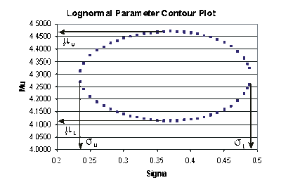
These points are represented graphically in the following contour plot:

(Note that this plot is generated with degrees of freedom [math]\displaystyle{ k=1 }[/math] , as we are only determining bounds on one parameter. The contour plots generated in Weibull++ are done with degrees of freedom [math]\displaystyle{ k=2 }[/math] , for use in comparing both parameters simultaneously.) As can be determined from the table the lowest calculated value for [math]\displaystyle{ {\mu }' }[/math] is 4.1145, while the highest is 4.4708. These represent the two-sided 75% confidence limits on this parameter. Since solutions for the equation do not exist for values of [math]\displaystyle{ {{\sigma' }} }[/math] below 0.24 or above 0.48, these can be considered the two-sided 75% confidence limits for this parameter. In order to obtain more accurate values for the confidence limits on [math]\displaystyle{ {{\sigma'}} }[/math] , we can perform the same procedure as before, but finding the two values of [math]\displaystyle{ \sigma }[/math] that correspond with a given value of [math]\displaystyle{ {\mu }'. }[/math] Using this method, we find that the 75% confidence limits on [math]\displaystyle{ {{\sigma'}} }[/math] are 0.23405 and 0.48936, which are close to the initial estimates of 0.24 and 0.48.