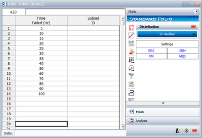
Template:Normal distribution rank regression on X
Rank Regression on X
As was mentioned previously, performing a rank regression on X requires that a straight line be fitted to a set of data points such that the sum of the squares of the horizontal deviations from the points to the fitted line is minimized.
Again, the first task is to bring our function, the probability of failure function for normal distribution, into a linear form. This step is exactly the same as in regression on Y analysis. All other equations apply in this case as they did for the regression on Y. The deviation from the previous analysis begins on the least squares fit step where: in this case, we treat [math]\displaystyle{ x }[/math] as the dependent variable and [math]\displaystyle{ y }[/math] as the independent variable. The best-fitting straight line for the data, for regression on X, is the straight line:
- [math]\displaystyle{ x=\widehat{a}+\widehat{b}y }[/math]
The corresponding equations for [math]\displaystyle{ \widehat{a} }[/math] and [math]\displaystyle{ \widehat{b} }[/math] are:
- [math]\displaystyle{ \hat{a}=\overline{x}-\hat{b}\overline{y}=\frac{\underset{i=1}{\overset{N}{\mathop{\sum }}}\,{{x}_{i}}}{N}-\hat{b}\frac{\underset{i=1}{\overset{N}{\mathop{\sum }}}\,{{y}_{i}}}{N} }[/math]
and:
- [math]\displaystyle{ \hat{b}=\frac{\underset{i=1}{\overset{N}{\mathop{\sum }}}\,{{x}_{i}}{{y}_{i}}-\tfrac{\underset{i=1}{\overset{N}{\mathop{\sum }}}\,{{x}_{i}}\underset{i=1}{\overset{N}{\mathop{\sum }}}\,{{y}_{i}}}{N}}{\underset{i=1}{\overset{N}{\mathop{\sum }}}\,y_{i}^{2}-\tfrac{{{\left( \underset{i=1}{\overset{N}{\mathop{\sum }}}\,{{y}_{i}} \right)}^{2}}}{N}} }[/math]
where:
- [math]\displaystyle{ {{y}_{i}}={{\Phi }^{-1}}\left[ F({{t}_{i}}) \right] }[/math]
and:
- [math]\displaystyle{ {{x}_{i}}={{t}_{i}} }[/math]
and the [math]\displaystyle{ F({{t}_{i}}) }[/math] values are estimated from the median ranks. Once [math]\displaystyle{ \widehat{a} }[/math] and [math]\displaystyle{ \widehat{b} }[/math] are obtained, solve the above linear equation for the unknown value of [math]\displaystyle{ y }[/math] which corresponds to:
- [math]\displaystyle{ y=-\frac{\widehat{a}}{\widehat{b}}+\frac{1}{\widehat{b}}x }[/math]
Solving for the parameters, we get:
- [math]\displaystyle{ a=-\frac{\widehat{a}}{\widehat{b}}=-\frac{\mu }{\sigma }\Rightarrow \mu =\widehat{a} }[/math]
and:
- [math]\displaystyle{ b=\frac{1}{\widehat{b}}=\frac{1}{\sigma }\Rightarrow \sigma =\widehat{b} }[/math]
The correlation coefficient is evaluated as before.
Example 3
Using the data of Example 2 and assuming a normal distribution, estimate the parameters and determine the correlation coefficient, [math]\displaystyle{ \rho }[/math] , using rank regression on X.
Solution to Example 3
Table 8.2 constructed in Example 2 applies to this example also. Using the values on this table, we get:
- [math]\displaystyle{ \begin{align} \hat{b}= & \frac{\underset{i=1}{\overset{14}{\mathop{\sum }}}\,{{T}_{i}}{{y}_{i}}-\tfrac{\underset{i=1}{\overset{14}{\mathop{\sum }}}\,{{T}_{i}}\underset{i=1}{\overset{14}{\mathop{\sum }}}\,{{y}_{i}}}{14}}{\underset{i=1}{\overset{14}{\mathop{\sum }}}\,y_{i}^{2}-\tfrac{{{\left( \underset{i=1}{\overset{14}{\mathop{\sum }}}\,{{y}_{i}} \right)}^{2}}}{14}} \\ \widehat{b}= & \frac{365.2711-(630)(0)/14}{11.3646-{{(0)}^{2}}/14}=32.1411 \end{align} }[/math]
- and:
- [math]\displaystyle{ \hat{a}=\overline{x}-\hat{b}\overline{y}=\frac{\underset{i=1}{\overset{14}{\mathop{\sum }}}\,{{T}_{i}}}{14}-\widehat{b}\frac{\underset{i=1}{\overset{14}{\mathop{\sum }}}\,{{y}_{i}}}{14} }[/math]
- or:
- [math]\displaystyle{ \widehat{a}=\frac{630}{14}-(32.1411)\frac{(0)}{14}=45 }[/math]
Therefore, from Eqn. (bnx):
- [math]\displaystyle{ \widehat{\sigma }=\widehat{b}=32.1411 }[/math]
- and from Eqn. (anx):
- [math]\displaystyle{ \widehat{\mu }=\widehat{a}=45\text{ hours} }[/math]
The correlation coefficient is found using Eqn. (RHOn):
- [math]\displaystyle{ \widehat{\rho }=0.979 }[/math]
Note that the results for regression on X are not necessarily the same as the results for regression on Y. The only time when the two regressions are the same (i.e. will yield the same equation for a line) is when the data lie perfectly on a straight line. Using Weibull++ , Rank Regression on X (RRX) can be selected from the Analysis page.
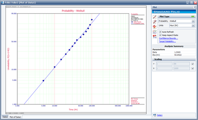
The plot of the solution for this example is shown next.
[math]\displaystyle{ }[/math]

