Template:Logistic confidence bounds

Confidence Bounds

In this section, we present the methods used in the application to estimate the different types of confidence bounds for logistically distributed data. The complete derivations were presented in detail (for a general function) in Chapter 5.

Bounds on the Parameters

The lower and upper bounds on the location parameter [math]\displaystyle{ \widehat{\mu } }[/math] are estimated from

[math]\displaystyle{ {{\mu }_{U}}=\widehat{\mu }+{{K}_{\alpha }}\sqrt{Var(\widehat{\mu })\text{ }}\text{ (upper bound)} }[/math]

[math]\displaystyle{ {{\mu }_{L}}=\widehat{\mu }-{{K}_{\alpha }}\sqrt{Var(\widehat{\mu })\text{ }}\text{ (lower bound)} }[/math]

The lower and upper bounds on the scale parameter [math]\displaystyle{ \widehat{\sigma } }[/math] are estimated from:

[math]\displaystyle{ {{\sigma }_{U}}=\widehat{\sigma }{{e}^{\tfrac{{{K}_{\alpha }}\sqrt{Var(\widehat{\sigma })\text{ }}}{\widehat{\sigma }}}}(\text{upper bound}) }[/math]

[math]\displaystyle{ {{\sigma }_{L}}=\widehat{\sigma }{{e}^{\tfrac{-{{K}_{\alpha }}\sqrt{Var(\widehat{\sigma })\text{ }}}{\widehat{\sigma }}}}\text{ (lower bound)} }[/math]

where [math]\displaystyle{ {{K}_{\alpha }} }[/math] is defined by:

[math]\displaystyle{ \alpha =\frac{1}{\sqrt{2\pi }}\int_{{{K}_{\alpha }}}^{\infty }{{e}^{-\tfrac{{{t}^{2}}}{2}}}dt=1-\Phi ({{K}_{\alpha }}) }[/math]

If [math]\displaystyle{ \delta }[/math] is the confidence level, then [math]\displaystyle{ \alpha =\tfrac{1-\delta }{2} }[/math] for the two-sided bounds, and [math]\displaystyle{ \alpha =1-\delta }[/math] for the one-sided bounds.

The variances and covariances of [math]\displaystyle{ \widehat{\mu } }[/math] and [math]\displaystyle{ \widehat{\sigma } }[/math] are estimated from the Fisher matrix, as follows:

[math]\displaystyle{ \left( \begin{matrix} \widehat{Var}\left( \widehat{\mu } \right) & \widehat{Cov}\left( \widehat{\mu },\widehat{\sigma } \right) \\ \widehat{Cov}\left( \widehat{\mu },\widehat{\sigma } \right) & \widehat{Var}\left( \widehat{\sigma } \right) \\ \end{matrix} \right)=\left( \begin{matrix} -\tfrac{{{\partial }^{2}}\Lambda }{\partial {{\mu }^{2}}} & -\tfrac{{{\partial }^{2}}\Lambda }{\partial \mu \partial \sigma } \\ {} & {} \\ -\tfrac{{{\partial }^{2}}\Lambda }{\partial \mu \partial \sigma } & -\tfrac{{{\partial }^{2}}\Lambda }{\partial {{\sigma }^{2}}} \\ \end{matrix} \right)_{\mu =\widehat{\mu },\sigma =\widehat{\sigma }}^{-1} }[/math]

[math]\displaystyle{ \Lambda }[/math] is the log-likelihood function of the normal distribution, described in Chapter 3 and Appendix C.

Bounds on Reliability

The reliability of the logistic distribution is:

[math]\displaystyle{ \widehat{R}=\frac{1}{1+{{e}^{\widehat{z}}}} }[/math]

where:

[math]\displaystyle{ \widehat{z}=\frac{T-\widehat{\mu }}{\widehat{\sigma }} }[/math]

Here [math]\displaystyle{ -\infty \lt T\lt \infty }[/math] , [math]\displaystyle{ -\infty \lt \mu \lt \infty }[/math] , [math]\displaystyle{ 0\lt \sigma \lt \infty }[/math] . Therefore, [math]\displaystyle{ z }[/math] also is changing from [math]\displaystyle{ -\infty }[/math] to [math]\displaystyle{ +\infty }[/math] . Then the bounds on [math]\displaystyle{ z }[/math] are estimated from:

[math]\displaystyle{ {{z}_{U}}=\widehat{z}+{{K}_{\alpha }}\sqrt{Var(\widehat{z})\text{ }} }[/math]

[math]\displaystyle{ {{z}_{L}}=\widehat{z}-{{K}_{\alpha }}\sqrt{Var(\widehat{z})\text{ }}\text{ } }[/math]

where:

[math]\displaystyle{ Var(\widehat{z})={{(\frac{\partial z}{\partial \mu })}^{2}}Var(\widehat{\mu })+2(\frac{\partial z}{\partial \mu })(\frac{\partial z}{\partial \sigma })Cov(\widehat{\mu },\widehat{\sigma })+{{(\frac{\partial z}{\partial \sigma })}^{2}}Var(\widehat{\sigma }) }[/math]

or:

[math]\displaystyle{ Var(\widehat{z})=\frac{1}{{{\sigma }^{2}}}(Var(\widehat{\mu })+2\widehat{z}Cov(\widehat{\mu },\widehat{\sigma })+{{\widehat{z}}^{2}}Var(\widehat{\sigma })) }[/math]

The upper and lower bounds on reliability are:

[math]\displaystyle{ {{R}_{U}}=\frac{1}{1+{{e}^{{{z}_{L}}}}}\text{(upper bound)} }[/math]

[math]\displaystyle{ {{R}_{L}}=\frac{1}{1+{{e}^{{{z}_{U}}}}}\text{(lower bound)} }[/math]

Bounds on Time

The bounds around time for a given logistic percentile (unreliability) are estimated by first solving the reliability equation with respect to time as follows:

[math]\displaystyle{ \widehat{T}(\widehat{\mu },\widehat{\sigma })=\widehat{\mu }+\widehat{\sigma }z }[/math]

where:

[math]\displaystyle{ z=\ln (1-R)-\ln (R) }[/math]

[math]\displaystyle{ Var(\widehat{T})={{(\frac{\partial T}{\partial \mu })}^{2}}Var(\widehat{\mu })+2(\frac{\partial T}{\partial \mu })(\frac{\partial T}{\partial \sigma })Cov(\widehat{\mu },\widehat{\sigma })+{{(\frac{\partial T}{\partial \sigma })}^{2}}Var(\widehat{\sigma }) }[/math]

or:

[math]\displaystyle{ Var(\widehat{T})=Var(\widehat{\mu })+2\widehat{z}Cov(\widehat{\mu },\widehat{\sigma })+{{\widehat{z}}^{2}}Var(\widehat{\sigma }) }[/math]

The upper and lower bounds are then found by:

[math]\displaystyle{ {{T}_{U}}=\widehat{T}+{{K}_{\alpha }}\sqrt{Var(\widehat{T})\text{ }}(\text{upper bound}) }[/math]

[math]\displaystyle{ {{T}_{L}}=\widehat{T}-{{K}_{\alpha }}\sqrt{Var(\widehat{T})\text{ }}(\text{lower bound}) }[/math]

A Logistic Distribution Example

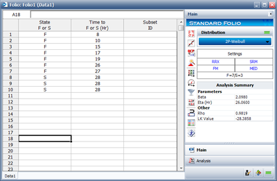
The lifetime of a mechanical valve is known to follow a logistic distribution. Ten units were tested for 28 months and the following months-to-failure data was collected.

[math]\displaystyle{ \overset{{}}{\mathop{\text{Table 10}\text{.1 - Times-to-Failure Data with Suspensions}}}\, }[/math] [math]\displaystyle{ \begin{matrix} \text{Data Point Index} & \text{State F or S} & \text{State End Time} \\ \text{1} & \text{F} & \text{8} \\ \text{2} & \text{F} & \text{10} \\ \text{3} & \text{F} & \text{15} \\ \text{4} & \text{F} & \text{17} \\ \text{5} & \text{F} & \text{19} \\ \text{6} & \text{F} & \text{26} \\ \text{7} & \text{F} & \text{27} \\ \text{8} & \text{S} & \text{28} \\ \text{9} & \text{S} & \text{28} \\ \text{10} & \text{S} & \text{28} \\ \end{matrix} }[/math]

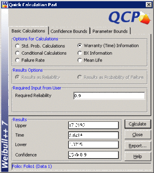
• Determine the valve's design life if specifications call for a reliability goal of 0.90.

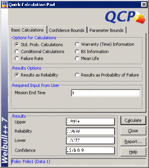
• The valve is to be used in a pumping device that requires 1 month of continuous operation. What is the probability of the pump failing due to the valve?

This data set can be entered into Weibull++ as follows:

The computed parameters for maximum likelihood are:

[math]\displaystyle{ \begin{align} & \widehat{\mu }= & 22.34 \\ & \hat{\sigma }= & 6.15 \end{align} }[/math]

• The valve's design life, along with 90% two sided confidence bounds, can be obtained using the QCP as follows:

• The probability, along with 90% two sided confidence bounds, that the pump fails due to a valve failure during the first month is obtained as follows: