Accelerated Life Testing and ALTA
Accelerated Life Testing and ALTA
This chapter presents issues relevant to using the ALTA software package to analyze data collected in accelerated life tests. These issues include the types of data that can be analyzed and the types of plots that can be created to display analysis results.
Residual Plots
Residual analysis for reliability consists of analyzing the results of a regression analysis by assigning residual values to each data point in the data set. Plotting these residuals provides a very good tool in assessing model assumptions and revealing inadequacies in the model, as well as revealing extreme observations. Three types of residual plots are available in ALTA.
Standardized Residuals (SR)
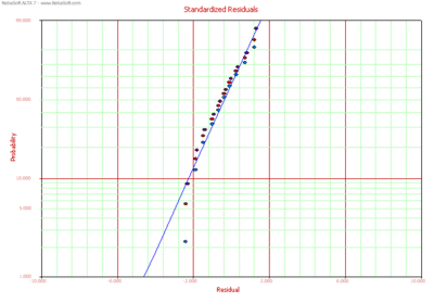
The standardized residuals plot for the Weibull and lognormal distributions can be obtained in ALTA. Each plot type is discussed next.
SR for the Weibull Distribution
Once the parameters have been estimated, the standardized residuals for the Weibull distribution can be calculated by:
- [math]\displaystyle{ {{\widehat{e}}_{i}}=\widehat{\beta }\left[ \ln ({{T}_{i}})-\ln (\widehat{\eta }(V)) \right] }[/math]
Then, under the assumed model, these residuals should look like a sample from an extreme value distribution with a mean of 0. For the Weibull distribution the standardized residuals are plotted on a smallest extreme value probability paper. If the Weibull distribution adequately describes the data, then the standardized residuals should appear to follow a straight line on such a probability plot. Note that when an observation is censored (suspended), the corresponding residual is also censored.
SR for the Lognormal Distribution
Once the parameters have been estimated using rank regression, the fitted or calculated responses can be calculated by:
- [math]\displaystyle{ {{\widehat{e}}_{i}}=\frac{\ln ({{T}_{i}})-{{\widehat{\mu }}^{\prime }}}{{{\widehat{\sigma }}_{{{T}'}}}} }[/math]
Then, under the assumed model, the standardized residuals should be normally distributed with a mean of 0 and a standard deviation of 1 ( [math]\displaystyle{ \tilde{\ }N(0,1) }[/math] ). Consequently, the standardized residuals for the lognormal distribution are commonly displayed on a normal probability plot.
Cox-Snell Residuals
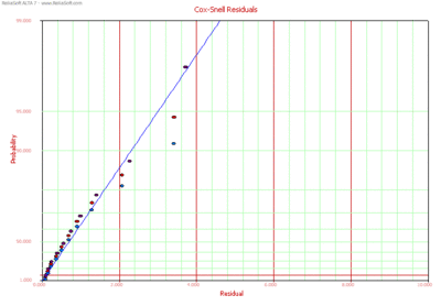
The Cox-Snell residuals are given by:
- [math]\displaystyle{ {{\widehat{e}}_{i}}=-\ln [R({{T}_{i}})] }[/math]
where [math]\displaystyle{ R({{T}_{i}}) }[/math] is the calculated reliability value at failure time [math]\displaystyle{ {{T}_{i}}. }[/math] The Cox-Snell residuals are plotted on an exponential probability paper.
- [math]\displaystyle{ }[/math]
Standardized vs Fitted Values
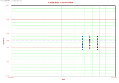
A Standardized vs. Fitted Value plot helps to detect behavior not modeled in the underlying relationship. However, when heavy censoring is present, the plot is more difficult to interpret. In a Standardized vs. Fitted Value plot, the standardized residuals are plotted versus the scale parameter of the underlying life distribution (which is a function of stress) on log-linear paper (linear on the Y-axis). Therefore, in the case of the Weibull distribution, the standardized residuals are plotted versus [math]\displaystyle{ \eta (V), }[/math] for the lognormal versus [math]\displaystyle{ {\mu }'(V), }[/math] and for the exponential versus [math]\displaystyle{ m(V). }[/math]
| The material on this page is copyrighted. | ©1992-2012. ReliaSoft Corporation. ALL RIGHTS RESERVED. |


