Competing Failure Modes Analysis

Competing Failure Modes

Often, a group of products will fail due to more than one failure mode. One can take the view that the products could have failed due to any one of the possible failure modes, but since an item cannot fail more than one time, there can only be one failure mode for each failed product. In this view, the failure modes compete as to which causes the failure for each particular item. This can be viewed as a series system reliability model, with each failure mode composing a block of the series system. Competing failure modes analysis segregates the analyses of failure modes and then combines the results to provide an overall model for the product in question.

In order to begin analyzing data sets with more than one competing failure mode, one must perform a separate analysis for each failure mode. During each of these analyses, the failure times for all other failure modes not being analyzed are considered to be suspensions. This is because the units under test would have failed at some time in the future due to the failure mode being analyzed, had the unrelated (not analyzed) mode not occurred. Thus, in this case, the information available is that the mode under consideration did not occur and the unit under consideration accumulated test time without a failure due to the mode under consideration (or a suspension due to that mode).

Once the analysis for each separate failure mode has been completed (using the same principles as before), the resulting reliability equation for all modes is the product of the reliability equation for each mode, or:

[math]\displaystyle{ R(t)={{R}_{1}}(t)\cdot {{R}_{2}}(t)\cdot ...\cdot {{R}_{n}}(t) }[/math]

where [math]\displaystyle{ n }[/math] is the total number of failure modes considered. This is the product rule for the reliability of series systems with statistically independent components, which states that the reliability for a series system is equal to the product of the reliability values of the components comprising the system. Do note that in Eqn. (sysrel) is the reliability function based on any assumed life distribution. In Weibull++ this life distribution can be either the 2-parameter Weibull, lognormal, normal or the 1-parameter exponential.

Example 13

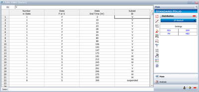
From Meeker & Escobar [27], the following table gives failure times for an electric component that has two failure modes.

One failure mode is due to random voltage spikes which cause failure by overloading the system (denoted as a [math]\displaystyle{ V }[/math] in the table). The other failure mode is due to wear-out failures which usually happen only after the system has run for many cycles (this failure mode is denoted as a [math]\displaystyle{ W }[/math] in the table).

Considering that these are competing failure modes, determine the overall reliability for the component at 100,000 cycles.

[math]\displaystyle{ \begin{matrix} Number & Failure & Failure & Number & Failure & Failure \\ in State & Time* & Mode & in State & Time* & Mode \\ \text{1} & \text{2} & \text{V} & \text{1} & \text{147} & \text{W} \\ \text{1} & \text{10} & \text{V} & \text{1} & \text{173} & \text{V} \\ \text{1} & \text{13} & \text{V} & \text{1} & \text{181} & \text{W} \\ \text{2} & \text{23} & \text{V} & \text{1} & \text{212} & \text{W} \\ \text{1} & \text{28} & \text{V} & \text{1} & \text{245} & \text{W} \\ \text{1} & \text{30} & \text{V} & \text{1} & \text{247} & \text{V} \\ \text{1} & \text{65} & \text{V} & \text{1} & \text{261} & \text{V} \\ \text{1} & \text{80} & \text{V} & \text{1} & \text{266} & \text{W} \\ \text{1} & \text{88} & \text{V} & \text{1} & \text{275} & \text{W} \\ \text{1} & \text{106} & \text{V} & \text{1} & \text{293} & \text{W} \\ \text{1} & \text{143} & \text{V} & \text{8} & \text{300} & \text{suspended} \\ \end{matrix} }[/math]

• Failure times given are in thousands of cycles.

Solution to Example 13

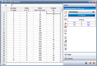
We will begin by performing a Weibull analysis of the voltage spike ( [math]\displaystyle{ V }[/math] ) failure mode. In order to do this, we must consider all of the failures for the wear-out mode to be suspensions. The input data for the analysis are shown next:

Analyzing this data set using the maximum likelihood method (recommended due to the number of suspensions in the data) and assuming a Weibull distribution, we obtain the parameters [math]\displaystyle{ {{\beta }_{V}}=0.6711 }[/math] and [math]\displaystyle{ {{\eta }_{V}}=449.4 }[/math] . The reliability for this failure mode at [math]\displaystyle{ t=100 }[/math] is [math]\displaystyle{ {{R}_{V}}(100)=0.694 }[/math] .

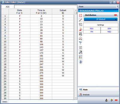
We follow an identical procedure for the wear-out failure mode, counting only the [math]\displaystyle{ W }[/math] entries as failures and assuming the [math]\displaystyle{ V }[/math] entries are suspensions. This is shown next.

Once again, analyzing with a Weibull distribution with maximum likelihood estimators, we obtain the parameters [math]\displaystyle{ {{\beta }_{W}}=4.337 }[/math] and [math]\displaystyle{ {{\eta }_{W}}=340.4 }[/math] . The reliability for this failure mode at [math]\displaystyle{ t=100 }[/math] is [math]\displaystyle{ {{R}_{W}}(100)=0.995 }[/math] .

We can now use Eqn. (sysrel) to determine the overall system reliability at 100,000 cycles:

[math]\displaystyle{ \begin{align} & {{R}_{sys}}(100)= & {{R}_{V}}(100)\cdot {{R}_{W}}(100) \\ & = & 0.694\cdot 0.995 \\ & = & 0.69053 \end{align} }[/math]

Or the reliability of the unit (or system) under both modes is [math]\displaystyle{ {{R}_{sys}}(100)=69.053%. }[/math]

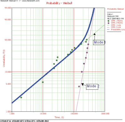
Note that Weibull++ can perform this analysis for you automatically. To accomplish this, the data would be entered in a single data sheet and competing failure modes chosen as the analysis method. This is shown in the next graphic.

Plotting Competing Failure Modes

[math]\displaystyle{ }[/math]

When plotting competing failure modes in Weibull++, your plots can contain the combined mode line as well as the individual mode lines. The User's Guide describes how these options can be turned on or off.

Confidence Bounds for Competing Failure Modes

The method available in Weibull++ for estimating the different types of confidence bounds, for competing failure modes analysis, is the Fisher matrix method, and is presented in this section.

Variance/Covariance Matrix

The variances and covariances of the parameters are estimated from the inverse local Fisher matrix, as follows:

[math]\displaystyle{ \begin{align} & & \left( \begin{matrix} Var\left( {{\widehat{a}}_{1}} \right) & Cov\left( {{\widehat{a}}_{1}},{{\widehat{b}}_{1}} \right) & 0 & 0 & 0 & 0 & 0 \\ Cov\left( {{\widehat{a}}_{1}},{{\widehat{b}}_{1}} \right) & Var\left( {{\widehat{b}}_{1}} \right) & 0 & 0 & 0 & 0 & 0 \\ 0 & 0 & . & 0 & 0 & 0 & 0 \\ 0 & 0 & 0 & . & 0 & 0 & 0 \\ 0 & 0 & 0 & 0 & . & 0 & 0 \\ 0 & 0 & 0 & 0 & 0 & Var\left( {{\widehat{a}}_{n}} \right) & Cov\left( {{\widehat{a}}_{n}},{{\widehat{b}}_{n}} \right) \\ 0 & 0 & 0 & 0 & 0 & Cov\left( {{\widehat{a}}_{n}},{{\widehat{b}}_{n}} \right) & Var\left( {{\widehat{b}}_{n}} \right) \\ \end{matrix} \right) \\ & & \\ & = & {{\left( \begin{matrix} -\tfrac{{{\partial }^{2}}\Lambda }{\partial a_{1}^{2}} & -\tfrac{{{\partial }^{2}}\Lambda }{\partial {{a}_{1}}\partial {{b}_{1}}} & 0 & 0 & 0 & 0 & 0 \\ -\tfrac{{{\partial }^{2}}\Lambda }{\partial {{a}_{1}}\partial {{b}_{1}}} & -\tfrac{{{\partial }^{2}}\Lambda }{\partial a_{1}^{2}} & 0 & 0 & 0 & 0 & 0 \\ 0 & 0 & . & 0 & 0 & 0 & 0 \\ 0 & 0 & 0 & . & 0 & 0 & 0 \\ 0 & 0 & 0 & 0 & . & 0 & 0 \\ 0 & 0 & 0 & 0 & 0 & -\tfrac{{{\partial }^{2}}\Lambda }{\partial a_{n}^{2}} & -\tfrac{{{\partial }^{2}}\Lambda }{\partial {{a}_{n}}\partial {{b}_{n}}} \\ 0 & 0 & 0 & 0 & 0 & -\tfrac{{{\partial }^{2}}\Lambda }{\partial {{a}_{n}}\partial {{b}_{n}}} & -\tfrac{{{\partial }^{2}}\Lambda }{\partial a_{n}^{2}} \\ \end{matrix} \right)}^{-1}} \end{align} }[/math]

where [math]\displaystyle{ \Lambda }[/math] is the log-likelihood function of the failure distribution, described in Chapter 5.

Bounds on Reliability

The competing failure modes reliability function is given by:

[math]\displaystyle{ \widehat{R}=\underset{i=1}{\overset{n}{\mathop \prod }}\,{{\hat{R}}_{i}} }[/math]

where:

• [math]\displaystyle{ {{R}_{i}} }[/math] is the reliability of the [math]\displaystyle{ {{i}^{th}} }[/math] mode,

• [math]\displaystyle{ n }[/math] is the number of failure modes.

The upper and lower bounds on reliability are estimated using the logit transformation:

[math]\displaystyle{ \begin{align} & {{R}_{U}}= & \frac{\widehat{R}}{\widehat{R}+(1-\widehat{R}){{e}^{-\tfrac{{{K}_{\alpha }}\sqrt{Var(\widehat{R})}}{\widehat{R}(1-\widehat{R})}}}} \\ & {{R}_{L}}= & \frac{\widehat{R}}{\widehat{R}+(1-\widehat{R}){{e}^{\tfrac{{{K}_{\alpha }}\sqrt{Var(\widehat{R})}}{\widehat{R}(1-\widehat{R})}}}} \end{align} }[/math]

where [math]\displaystyle{ \widehat{R} }[/math] is calculated using Eqn. (CFMReliability). [math]\displaystyle{ {{K}_{\alpha }} }[/math] is defined by:

[math]\displaystyle{ \alpha =\frac{1}{\sqrt{2\pi }}\underset{{{K}_{\alpha }}}{\overset{\infty }{\mathop \int }}\,{{e}^{-\tfrac{{{t}^{2}}}{2}}}dt=1-\Phi ({{K}_{\alpha }}) }[/math]

(If [math]\displaystyle{ \delta }[/math] is the confidence level, then [math]\displaystyle{ \alpha =\tfrac{1-\delta }{2} }[/math] for the two-sided bounds, and [math]\displaystyle{ \alpha =1-\delta }[/math] for the one-sided bounds.)

The variance of [math]\displaystyle{ \widehat{R} }[/math] is estimated by:

[math]\displaystyle{ Var(\widehat{R})=\underset{i=1}{\overset{n}{\mathop \sum }}\,{{\left( \frac{\partial R}{\partial {{R}_{i}}} \right)}^{2}}Var({{\hat{R}}_{i}}) }[/math]

[math]\displaystyle{ \frac{\partial R}{\partial {{R}_{i}}}=\underset{j=1,j\ne i}{\overset{n}{\mathop \prod }}\,\widehat{{{R}_{j}}} }[/math]

Thus:

[math]\displaystyle{ Var(\widehat{R})=\underset{i=1}{\overset{n}{\mathop \sum }}\,\left( \underset{j=1,j\ne i}{\overset{n}{\mathop \prod }}\,\widehat{R}_{j}^{2} \right)Var({{\hat{R}}_{i}}) }[/math]

[math]\displaystyle{ Var({{\hat{R}}_{i}})=\underset{i=1}{\overset{n}{\mathop \sum }}\,{{\left( \frac{\partial {{R}_{i}}}{\partial {{a}_{i}}} \right)}^{2}}Var({{\hat{a}}_{i}}) }[/math]

where [math]\displaystyle{ \widehat{{{a}_{i}}} }[/math] is an element of the model parameter vector.

Therefore, the value of [math]\displaystyle{ Var({{\hat{R}}_{i}}) }[/math] is dependent on the underlying distribution.

For the Weibull distribution:

[math]\displaystyle{ Var({{\hat{R}}_{i}})={{\left( {{{\hat{R}}}_{i}}{{e}^{{{{\hat{u}}}_{i}}}} \right)}^{2}}Var({{\hat{u}}_{i}}) }[/math]

where:

[math]\displaystyle{ {{\hat{u}}_{i}}={{\hat{\beta }}_{i}}(\ln (t-{{\hat{\gamma }}_{i}})-\ln {{\hat{\eta }}_{i}}) }[/math]

and [math]\displaystyle{ Var(\widehat{{{u}_{i}}}) }[/math] is given in Chapter 6.

For the exponential distribution:

[math]\displaystyle{ Var({{\hat{R}}_{i}})={{\left( {{{\hat{R}}}_{i}}(t-{{{\hat{\gamma }}}_{i}}) \right)}^{2}}Var({{\hat{\lambda }}_{i}}) }[/math]

where [math]\displaystyle{ Var(\widehat{{{\lambda }_{i}}}) }[/math] is given in Chapter 7.

For the normal distribution:

[math]\displaystyle{ Var({{\hat{R}}_{i}})={{\left( f({{{\hat{z}}}_{i}})\hat{\sigma } \right)}^{2}}Var({{\hat{z}}_{i}}) }[/math]

[math]\displaystyle{ {{\hat{z}}_{i}}=\frac{t-{{{\hat{\mu }}}_{i}}}{{{{\hat{\sigma }}}_{i}}} }[/math]

where [math]\displaystyle{ Var(\widehat{{{z}_{i}}}) }[/math] is given in Chapter 8.

For the lognormal distribution:

[math]\displaystyle{ Var({{\hat{R}}_{i}})={{\left( f({{{\hat{z}}}_{i}})\cdot {{{\hat{\sigma }}}^{\prime }} \right)}^{2}}Var({{\hat{z}}_{i}}) }[/math]

[math]\displaystyle{ {{\hat{z}}_{i}}=\frac{\ln \text{(}t)-\hat{\mu }_{i}^{\prime }}{\hat{\sigma }_{i}^{\prime }} }[/math]

where [math]\displaystyle{ Var(\widehat{{{z}_{i}}}) }[/math] is given in Chapter 9.

Bounds on Time

The bounds on time are estimate by solving the reliability equation with respect to time. From Eqn. (CFMReliability) we have that:

[math]\displaystyle{ \hat{t}=\varphi (R,{{\hat{a}}_{i}},{{\hat{b}}_{i}}) }[/math]

[math]\displaystyle{ i=1,...,n }[/math]

where:

• [math]\displaystyle{ \varphi }[/math] is inverse function for Eqn. (CFMReliability)

• for the Weibull distribution [math]\displaystyle{ {{\hat{a}}_{i}} }[/math] is [math]\displaystyle{ {{\hat{\beta }}_{i}} }[/math] , and [math]\displaystyle{ {{\hat{b}}_{i}} }[/math] is [math]\displaystyle{ {{\hat{\eta }}_{i}} }[/math]

• for the exponential distribution [math]\displaystyle{ {{\hat{a}}_{i}} }[/math] is [math]\displaystyle{ {{\hat{\lambda }}_{i}} }[/math] , and [math]\displaystyle{ {{\hat{b}}_{i}} }[/math] =0

• for the normal distribution [math]\displaystyle{ {{\hat{a}}_{i}} }[/math] is [math]\displaystyle{ {{\hat{\mu }}_{i}} }[/math] , and [math]\displaystyle{ {{\hat{b}}_{i}} }[/math] is [math]\displaystyle{ {{\hat{\sigma }}_{i}} }[/math] , and

• for the lognormal distribution [math]\displaystyle{ {{\hat{a}}_{i}} }[/math] is [math]\displaystyle{ \hat{\mu }_{i}^{\prime } }[/math] , and [math]\displaystyle{ {{\hat{b}}_{i}} }[/math] is [math]\displaystyle{ \hat{\sigma }_{i}^{\prime } }[/math]

Set:

[math]\displaystyle{ u=\ln (t) }[/math]

The bounds on [math]\displaystyle{ u }[/math] are estimated from:

[math]\displaystyle{ {{u}_{U}}=\widehat{u}+{{K}_{\alpha }}\sqrt{Var(\widehat{u})} }[/math]

and:

[math]\displaystyle{ {{u}_{L}}=\widehat{u}-{{K}_{\alpha }}\sqrt{Var(\widehat{u})} }[/math]

Then the upper and lower bounds on time are found by using the equations

[math]\displaystyle{ {{t}_{U}}={{e}^{{{u}_{U}}}} }[/math]

and:

[math]\displaystyle{ {{t}_{L}}={{e}^{{{u}_{L}}}} }[/math]

[math]\displaystyle{ {{K}_{\alpha }} }[/math] is calculated using Eqn. (ka) and [math]\displaystyle{ Var(\widehat{u}) }[/math] is computed as:

[math]\displaystyle{ Var(\widehat{u})=\underset{i=1}{\overset{n}{\mathop \sum }}\,\left( {{\left( \frac{\partial u}{\partial {{a}_{i}}} \right)}^{2}}Var(\widehat{{{a}_{i}}})+{{\left( \frac{\partial u}{\partial {{b}_{i}}} \right)}^{2}}Var(\widehat{{{b}_{i}}})+2\frac{\partial u}{\partial {{a}_{i}}}\frac{\partial u}{\partial {{b}_{i}}}Cov(\widehat{{{a}_{i}}},\widehat{{{b}_{i}}}) \right) }[/math]

Complex Competing Failure Modes

In addition to being viewed as a series system, the relationship between the different competing failures modes can be more complex. After performing separate analysis for each failure mode, a diagram that describes how each failure mode can result in a product failure can be used to perform analysis for the item in question. Such diagrams are usually referred to as Reliability Block Diagrams (RBD) (for more on RBDs see ReliaSoft's System Analysis Reference and ReliaSoft's BlockSim software).

A reliability block diagram is made of blocks that represent the failure modes and arrows and connects the blocks in different configurations. Note that the blocks can also be used to represent different components or subsystems that make up the product. Weibull ++ provides the capability to use a diagram to model, series, parallel, k-out-of-n configurations in addition to any complex combinations of these configurations.

In this analysis, the failure modes are assumed to be statistically independent. (Note: In the context of this reference, statistically independent implies that failure information for one failure mode provides no information about, i.e. does not affect, other failure mode). Analysis of dependent modes is more complex. Advanced RBD software such as ReliaSoft's BlockSim can handle and analyze such dependencies, as well as provide more advanced constructs and analyses (see http://www.reliasoft.com/BlockSim).

Failure Modes Configurations

Series Configuration

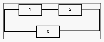
The basic competing failure modes configuration, which has already been discussed, is a series configuration. In a series configuration, the occurrence of any failure mode results in failure for the product.

The equation that describes series configuration is:

[math]\displaystyle{ R(t)={{R}_{1}}(t)\cdot {{R}_{2}}(t)\cdot ...\cdot {{R}_{n}}(t) }[/math]

where [math]\displaystyle{ n }[/math] is the total number of failure modes considered.

Parallel

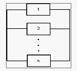
In a simple parallel configuration, at least one of the failure modes must not occur for the product to continue operation.

[math]\displaystyle{ }[/math]

The equation that describes parallel configuration is:

[math]\displaystyle{ R(t)=1-\underset{i=1}{\overset{n}{\mathop \prod }}\,(1-{{R}_{i}}(t)) }[/math]

where [math]\displaystyle{ n }[/math] is the total number of failure modes considered.

Combination of Series and Parallel

While many smaller products can be accurately represented by either a simple series or parallel configuration, there may be larger products that involve both series and parallel configurations in the overall model of the product. Such products can be analyzed by calculating the reliabilities for the individual series and parallel sections and then combining them in the appropriate manner.

[math]\displaystyle{ }[/math]

k-out-of-n Parallel Configuration

The k-out-of-n configuration is a special case of parallel redundancy. This type of configuration requires that at least [math]\displaystyle{ k }[/math] failure modes do not happen out of the total [math]\displaystyle{ n }[/math] parallel failure modes for the product to succeed. The simplest case of a k-out-of-n configuration is when the failure modes are independent and identical and have the same failure distribution and uncertainties about the parameters (in other words they are derived from the same test data). In this case, the reliability of the product with such a configuration can be evaluated using the binomial distribution, or:

[math]\displaystyle{ R(t)=\overset{n}{\mathop{\underset{r=k}{\mathop{\underset{}{\overset{}{\mathop \sum }}\,}}\,}}\,\left( \underset{k}{\mathop{\overset{n}{\mathop{{}}}\,}}\, \right){{R}^{r}}(t){{(1-R(t))}^{n-r}} }[/math]

In the case where the k-out-of-n failure modes are not identical, other approaches for calculating the reliability must be used (e.g. the event space method). Discussion of these is beyond the scope of this reference. Interested readers can consult ReliaSoft's System Reliability Reference.

Complex Systems

In many cases, it is not easy to recognize which components are in series and which are in parallel in a complex system.

The previous configuration cannot be broken down into a group of series and parallel configurations. This is primarily due to the fact that failure mode C has two paths leading away from it, whereas B and D have only one. Several methods exist for obtaining the reliability of a complex configuration including the decomposition method, the event space method and the path-tracing method. Discussion of these is beyond the scope of this reference. Interested readers can consult ReliaSoft's System Reliability Reference.

Example 14

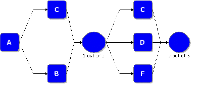
Assume that a product has five failure modes: A, B, C, D and F. Furthermore, assume that failure of the product will occur if mode A occurs, modes B and C occur simultaneously or if either modes C and D, C and F or D and F occur simultaneously. Times-to-failure for each mode is given in the next table.

[math]\displaystyle{ \begin{matrix} \text{TTF for A} & \text{TTF for B} & \text{TTF for C} & \text{TTF for D} & \text{TTF for F} \\ \text{276} & \text{23} & \text{499} & \text{467} & \text{67} \\ \text{320} & \text{36} & \text{545} & \text{540} & \text{72} \\ \text{323} & \text{57} & \text{661} & \text{716} & \text{81} \\ \text{558} & \text{89} & \text{738} & \text{737} & \text{108} \\ \text{674} & \text{99} & \text{987} & \text{761} & \text{110} \\ \text{829} & \text{154} & \text{1165} & \text{1093} & \text{127} \\ \text{878} & \text{200} & \text{1337} & \text{1283} & \text{148} \\ \end{matrix} }[/math]

The RBD that describes this configuration is shown next.

[math]\displaystyle{ }[/math]

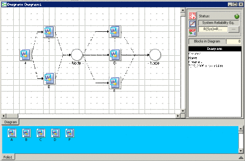
One folio with multiple data sheets was created in Weibull++ for each of the data sets and each file was analyzed using the two-parameter Weibull distribution, MLE as the analysis method and Fisher Matrix as the confidence bounds method. A diagram is created by choosing Add Diagram from the Project menu. The failure modes can be inserted into the diagram by dragging them from the template. The nodes are inserted by clicking choosing Add Node from the Diagram menu.

[math]\displaystyle{ }[/math]

The number of required paths can be specified by double clicking the node and entering the appropriate number (1 in the first node and 2 in the second node).

[math]\displaystyle{ }[/math]

Using the Quick Calculation Pad (QCP), the estimated R( [math]\displaystyle{ 100 }[/math] hours [math]\displaystyle{ ) }[/math] and the 90% two-sided confidence bounds are:

[math]\displaystyle{ \begin{matrix} {{{\hat{R}}}_{U}}(100)=0.991 \\ \hat{R}(100)=0.9905 \\ {{{\hat{R}}}_{L}}(100)=0.9080 \\ \end{matrix} }[/math]