Template:Recurrent events data analysis
Recurrent Events Data Analysis
Recurrent Events Data Analysis, also called Recurrence Data Analysis (RDA), can be used in various applied fields such as reliability, medicine, social sciences, economics, business and criminology.
Whereas in life data analysis (LDA) it was assumed that events (failures) were independent and identically distributed (iid), there are many cases where events are dependent and not identically distributed (such as repairable system data) or where the analyst is interested in modeling the number of occurrences of events over time rather than the length of time prior to the first event, as in LDA.
Weibull++ provides both parametric and non-parametric approaches to analyze such data.
- • The non-parametric approach is based on the well-known Mean Cumulative Function (MCF). The Weibull++ module for this type of analysis builds upon the work of Dr. Wayne Nelson, who has written extensively on the calculation and applications of MCF [31].
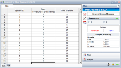
- • The parametric approach is based on the General Renewal Process (GRP) model, which is particularly useful in understanding the effects of the repairs on the age of a system. Traditionally, the commonly used models for analyzing repairable systems data are perfect renewal processes (PRP), corresponding to perfect repairs, and nonhomogeneous Poisson processes (NHPP), corresponding to minimal repairs. However, most repair activities may realistically not result in such extreme situations but in a complicated intermediate one (general repair or imperfect repair/maintenance), which are well treated with the GRP model.
Non-Parameteric Recurrence Data Analysis
Introduction
Non-parametric recurrence data analysis provides a nonparametric graphical estimate of the mean cumulative number or cost of recurrence per unit versus age. In the reliability field, the Mean Cumulative Function (MCF) can be used to: [31]
- • Evaluate whether the population repair (or cost) rate increases or decreases with age (this is useful for product retirement and burn-in decisions).
- • Estimate the average number or cost of repairs per unit during warranty or some time period.
- • Compare two or more sets of data from different designs, production periods, maintenance policies, environments, operating conditions, etc.
- • Predict future numbers and costs of repairs, such as, the next month, quarter, or year.
- • Reveal unexpected information and insight.
The Mean Cumulative Function (MCF) for Recurrence Data
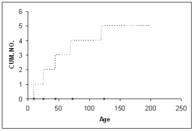
In non-parametric analysis of recurrent events data, each population unit can be described by a cumulative history function for the cumulative number of recurrences. It is a staircase function that depicts the cumulative number of recurrences of a particular event, such as repairs, over time. Figure CHM depicts a unit's cumulative history function.
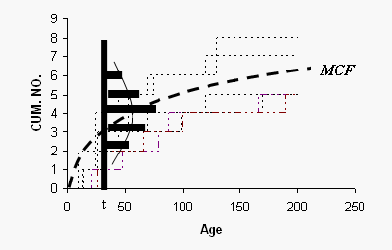
The nonparametric model for a population of units is described as the population of cumulative history functions (curves). It is the population of all staircase functions of every unit in the population. At age t, the units have a distribution of their cumulative number of events. That is, a fraction of the population has accumulated 0 recurrences, another fraction has accumulated 1 recurrence, another fraction has accumulated 2 recurrences, etc. This distribution differs at different ages, [math]\displaystyle{ t }[/math] , and has a mean [math]\displaystyle{ M(t) }[/math] called the mean cumulative function (MCF) . The [math]\displaystyle{ M(t) }[/math] is the pointwise average of all population cumulative history functions(see Fig.MCFDemo).
For the case of uncensored data, the mean cumulative function [math]\displaystyle{ M{{(t)}_{i}}\ }[/math] values at different recurrence ages [math]\displaystyle{ {{t}_{i}} }[/math] are estimated by calculating the average of the cumulative number of recurrences of events for each unit in the population at [math]\displaystyle{ {{t}_{i}} }[/math] . When the histories are censored, the following steps are applied.
1st Step - Order All Ages:
Order all recurrence and censoring ages from smallest to largest. If a recurrence age for a unit is the same as its censoring (suspension) age, the recurrence age goes first. If multiple units have a common recurrence or censoring age, then these units could be put in a certain order or be sorted randomly.
2nd Step - Calculate the Number, [math]\displaystyle{ {{r}_{i}} }[/math] , of Units that Passed Through Age [math]\displaystyle{ {{t}_{i}} }[/math] :
- [math]\displaystyle{ \begin{align} & {{r}_{i}}= & {{r}_{i-1}}\quad \quad \text{if }{{t}_{i}}\text{ is a recurrence age} \\ & {{r}_{i}}= & {{r}_{i-1}}-1\text{ if }{{t}_{i}}\text{ is a censoring age} \end{align} }[/math]
[math]\displaystyle{ N }[/math] is the total number of units and [math]\displaystyle{ {{r}_{1}}=N }[/math] at the first observed age which could be a recurrence or suspension.
3rd Step - Calculate [math]\displaystyle{ MCF }[/math] Estimate, [math]\displaystyle{ {{M}^{*}}(t) }[/math]: For each sample recurrence age [math]\displaystyle{ {{t}_{i}}, }[/math] calculate the mean cumulative function estimate as follows:
- [math]\displaystyle{ {{M}^{*}}({{t}_{i}})=\frac{1}{{{r}_{i}}}+{{M}^{*}}({{t}_{i-1}}) }[/math]
where [math]\displaystyle{ {{M}^{*}}(t)=\tfrac{1}{{{r}_{1}}} }[/math] at the earliest observed recurrence age, [math]\displaystyle{ {{t}_{1}} }[/math] .
Example 1
A health care company maintains five identical pieces of equipment used by a hospital. When a piece of equipment fails, the company sends a crew to repair it. The following table gives the failure and censoring ages for each machine, where the + sign indicates a censoring age.
[math]\displaystyle{ }[/math] Estimate the MCF values and the 95% confidence limits ignoring the repair duration.
Solution to Example 1
The MCF estimate is obtained as follows:
Confidence Limits for the MCF
Upper and lower conifidence limits for [math]\displaystyle{ M({{t}_{i}}) }[/math] are:
- [math]\displaystyle{ \begin{align} & {{M}_{U}}({{t}_{i}})= & {{M}^{*}}({{t}_{i}}).{{e}^{\tfrac{{{K}_{\alpha }}.\sqrt{Var[{{M}^{*}}({{t}_{i}})]}}{{{M}^{*}}({{t}_{i}})}}} \\ & {{M}_{L}}({{t}_{i}})= & \frac{{{M}^{*}}({{t}_{i}})}{{{e}^{\tfrac{{{K}_{\alpha }}.\sqrt{Var[{{M}^{*}}({{t}_{i}})]}}{{{M}^{*}}({{t}_{i}})}}}} \end{align} }[/math]
where [math]\displaystyle{ \alpha }[/math] ( [math]\displaystyle{ 50%\lt \alpha \lt 100% }[/math] ) is confidence level, [math]\displaystyle{ {{K}_{\alpha }} }[/math] is the [math]\displaystyle{ \alpha }[/math] standard normal percentile and [math]\displaystyle{ Var[{{M}^{*}}({{t}_{i}})] }[/math] is the variance of the MCF estimate at recurrence age [math]\displaystyle{ {{t}_{i}} }[/math] . The variance is calculated as follows:
- [math]\displaystyle{ Var[{{M}^{*}}({{t}_{i}})]=Var[{{M}^{*}}({{t}_{i-1}})]+\frac{1}{r_{i}^{2}}\left[ \underset{j\in {{R}_{i}}}{\overset{}{\mathop \sum }}\,{{\left( {{d}_{ji}}-\frac{1}{{{r}_{i}}} \right)}^{2}} \right] }[/math]
where [math]\displaystyle{ r }[/math] is defined in Eqn.(R), [math]\displaystyle{ {{R}_{i}} }[/math] is the set of the units that have not been suspended by [math]\displaystyle{ i }[/math] and [math]\displaystyle{ {{d}_{ji}} }[/math] is defined as follows:
- [math]\displaystyle{ \begin{align} & {{d}_{ji}}= & 1\text{ if the }{{j}^{\text{th }}}\text{unit had an event recurrence at age }{{t}_{i}} \\ & {{d}_{ji}}= & 0\text{ if the }{{j}^{\text{th }}}\text{unit did not have an event reoccur at age }{{t}_{i}} \end{align} }[/math]
Example 2
Using the data in Example 1, estimate the 95% confidence bounds.
Solution to Example 2
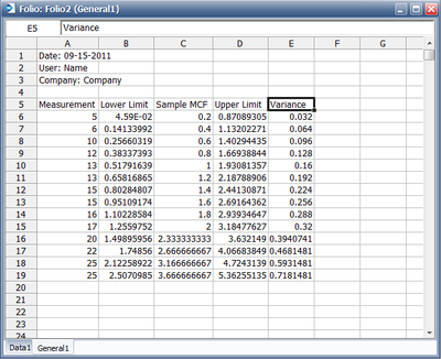
Using Eq. MCF Var the following table of variance values can be obtained:
| ID | Months | State | [math]\displaystyle{ r_i }[/math] | [math]\displaystyle{ Var_i }[/math] |
|---|---|---|---|---|
| 1 | 5 | F | 5 | [math]\displaystyle{ (\tfrac{1}{5})^2[(1-\tfrac{1}{5})^2+4(0-\tfrac{1}{5})^2]=0.032 }[/math] |
| 2 | 6 | F | 5 | [math]\displaystyle{ 0.032+(\tfrac{1}{5})^2[(1-\tfrac{1}{5})^2+4(0-\tfrac{1}{5})^2]=0.064 }[/math] |
| 1 | 10 | F | 5 | [math]\displaystyle{ 0.064+(\tfrac{1}{5})^2[(1-\tfrac{1}{5})^2+4(0-\tfrac{1}{5})^2]=0.096 }[/math] |
| 3 | 12 | F | 5 | [math]\displaystyle{ 0.096+(\tfrac{1}{5})^2[(1-\tfrac{1}{5})^2+4(0-\tfrac{1}{5})^2]=0.128 }[/math] |
| 2 | 13 | F | 5 | [math]\displaystyle{ 0.128+(\tfrac{1}{5})^2[(1-\tfrac{1}{5})^2+4(0-\tfrac{1}{5})^2]=0.160 }[/math] |
| 4 | 13 | F | 5 | [math]\displaystyle{ 0.160+(\tfrac{1}{5})^2[(1-\tfrac{1}{5})^2+4(0-\tfrac{1}{5})^2]=0.192 }[/math] |
| 1 | 15 | F | 5 | [math]\displaystyle{ 0.192+(\tfrac{1}{5})^2[(1-\tfrac{1}{5})^2+4(0-\tfrac{1}{5})^2]=0.224 }[/math] |
| 4 | 15 | F | 5 | [math]\displaystyle{ 0.224+(\tfrac{1}{5})^2[(1-\tfrac{1}{5})^2+4(0-\tfrac{1}{5})^2]=0.256 }[/math] |
| 5 | 16 | F | 5 | [math]\displaystyle{ 0.256+(\tfrac{1}{5})^2[3(0-\tfrac{1}{5})^2+2(1-\tfrac{1}{5})^2]=0.288 }[/math] |
| 2 | 17 | F | 5 | [math]\displaystyle{ 0.288+(\tfrac{1}{5})^2[(1-\tfrac{1}{5})^2+4(0-\tfrac{1}{5})^2]=0.320 }[/math] |
| 1 | 17 | S | 4 | |
| 2 | 19 | S | 3 | |
| 3 | 20 | F | 3 | [math]\displaystyle{ 0.320+(\tfrac{1}{5})^2[(1-\tfrac{1}{5})^2+2(0-\tfrac{1}{5})^2]=0.394 }[/math] |
| 5 | 22 | F | 3 | [math]\displaystyle{ 0.394+(\tfrac{1}{5})^2[2(0-\tfrac{1}{5})^2+4(1-\tfrac{1}{5})^2]=0.468 }[/math] |
| 4 | 24 | S | 2 | |
| 3 | 25 | F | 2 | [math]\displaystyle{ 0.468+(\tfrac{1}{5})^2[(1-\tfrac{1}{5})^2+4(0-\tfrac{1}{5})^2]=0.593 }[/math] |
| 5 | 25 | F | 2 | [math]\displaystyle{ 0.580+(\tfrac{1}{5})^2[(0-\tfrac{1}{5})^2+4(1-\tfrac{1}{5})^2]=0.718 }[/math] |
| 3 | 26 | S | 1 | |
| 5 | 28 | S | 0 |
Using Eqn.(MCF Bounds) and [math]\displaystyle{ {{K}_{5}}=1.644 }[/math] for a 95% confidence level, the confidence bounds can be obtained as follows:
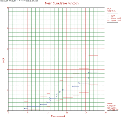
The analysis presented in Examples 1 and 2 can be obtained automatically in Weibull ++ using the Non-Parametric RDA Specialized Folio, as shown next.
Note: In the above Folio, the [math]\displaystyle{ F }[/math] refers to failures and [math]\displaystyle{ E }[/math] refers to suspensions (or censoring ages).
The results with calculated MCF values and upper and lower 95% confidence limits are shown next along with the graphical plot.
Example 3
The following table displays transmission repairs on a sample of 14 cars with manual transmission in a preproduction road test [31]. Here + denotes the censoring ages (how long a car has been observed).
The car manufacturer seeks to estimate the mean cumulative number of repairs per car by 24,000 test miles (equivalently 5.5 x 24,000 = 132,000 customer miles) and to observe whether the population repair rate increases or decreases as a population ages.
Solution to Example 3
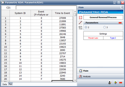
The data is entered into a Non-Parametric RDA Specialized Folio in Weibull++ as follows.
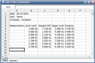
The results are as follows,
The results indicate that after 13,957 miles of testing, the estimated mean cumulative number of repairs per car is 0.5. Therefore, by 24,000 test miles, the estimated mean cumulative number of repairs per car is 0.5.
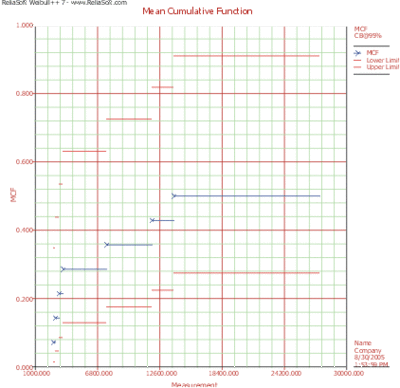
The MCF plot is shown next.
A smooth curve through the MCF plot has a derivative that decreases as the population ages. That is, the repair rate decreases as each population ages. This is typical of products with manufacturing defects.
