Template:Rank Regression or Least Squares Parameter Estimation
Rank Regression or Least Squares Parameter Estimation
Using the idea of probability plotting, regression analysis mathematically fits the best straight line to a set of points, in an attempt to estimate the parameters. Essentially, this is a mathematically based version of the probability plotting method discussed previously.
Background Theory
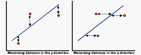
The method of linear least squares is used for all regression analysis performed by Weibull++, except for the cases of the three-parameter Weibull, mixed Weibull, gamma and generalized gamma distributions where a non-linear regression technique is employed. The terms linear regression and least squares are used synonymously in this reference. The term rank regression is used instead of least squares, or linear regression, because the regression is performed on the rank values, more specifically, the median rank values (represented on the y-axis). The method of least squares requires that a straight line be fitted to a set of data points, such that the sum of the squares of the distance of the points to the fitted line is minimized. This minimization can be performed in either the vertical or horizontal direction. If the regression is on [math]\displaystyle{ X }[/math], then the line is fitted so that the horizontal deviations from the points to the line are minimized. If the regression is on Y, then this means that the distance of the vertical deviations from the points to the line is minimized. This is illustrated in the following figure.
Rank Regression on [math]\displaystyle{ Y }[/math]
Assume that a set of data pairs [math]\displaystyle{ ({x_1},{y_1}) }[/math], [math]\displaystyle{ ({{x}_{2}},{{y}_{2}}) }[/math],..., [math]\displaystyle{ ({{x}_{N}},{{y}_{N}}) }[/math] were obtained and plotted, and that the [math]\displaystyle{ x }[/math] -values are known exactly. Then, according to the least squares principle, which minimizes the vertical distance between the data points and the straight line fitted to the data, the best fitting straight line to these data is the straight line [math]\displaystyle{ y=\hat{a}+\hat{b}x }[/math] (where the recently introduced [math]\displaystyle{ (\hat{ }) }[/math] symbol indicates that this value is an estimate) such that: .. and where [math]\displaystyle{ \hat{a} }[/math] and [math]\displaystyle{ \hat b }[/math] are the least squares estimates of [math]\displaystyle{ a }[/math] and [math]\displaystyle{ b }[/math],and [math]\displaystyle{ N }[/math] is the number of data points. These equations are minimized by estimates of [math]\displaystyle{ \widehat a }[/math] and [math]\displaystyle{ \widehat{b} }[/math] such that:
- [math]\displaystyle{ \hat{a}=\frac{\underset{i=1}{\overset{N}{\mathop{\sum }}}\,{{y}_{i}}}{N}-\hat{b}\frac{\underset{i=1}{\overset{N}{\mathop{\sum }}}\,{{x}_{i}}}{N}=\bar{y}-\hat{b}\bar{x} }[/math]
- and:
- [math]\displaystyle{ \hat{b}=\frac{\underset{i=1}{\overset{N}{\mathop{\sum }}}\,{{x}_{i}}{{y}_{i}}-\tfrac{\underset{i=1}{\overset{N}{\mathop{\sum }}}\,{{x}_{i}}\underset{i=1}{\overset{N}{\mathop{\sum }}}\,{{y}_{i}}}{N}}{\underset{i=1}{\overset{N}{\mathop{\sum }}}\,x_{i}^{2}-\tfrac{{{\left( \underset{i=1}{\overset{N}{\mathop{\sum }}}\,{{x}_{i}} \right)}^{2}}}{N}} }[/math]
Rank Regression on X
Assume that a set of data pairs .., [math]\displaystyle{ ({x_2},{y_2}) }[/math],..., [math]\displaystyle{ ({x_N},{y_N}) }[/math]were obtained and plotted, and that the y-values are known exactly. The same least squares principle is applied, this time minimizing the horizontal distance between the data points and the straight line fitted to the data. The best fitting straight line to these data is the straight line [math]\displaystyle{ x=\widehat{a}+\widehat{b}y }[/math] such that:
- [math]\displaystyle{ \underset{i=1}{\overset{N}{\mathop \sum }}\,{{(\widehat{a}+\widehat{b}{{y}_{i}}-{{x}_{i}})}^{2}}=min(a,b)\underset{i=1}{\overset{N}{\mathop \sum }}\,{{(a+b{{y}_{i}}-{{x}_{i}})}^{2}} }[/math]
Again, [math]\displaystyle{ \widehat{a} }[/math] and [math]\displaystyle{ \widehat b }[/math] are the least squares estimates of and [math]\displaystyle{ b, }[/math] and [math]\displaystyle{ N }[/math] is the number of data points. These equations are minimized by estimates of [math]\displaystyle{ \widehat a }[/math] and [math]\displaystyle{ \widehat{b} }[/math] such that:
- [math]\displaystyle{ \hat{a}=\frac{\underset{i=1}{\overset{N}{\mathop{\sum }}}\,{{x}_{i}}}{N}-\hat{b}\frac{\underset{i=1}{\overset{N}{\mathop{\sum }}}\,{{y}_{i}}}{N}=\bar{x}-\hat{b}\bar{y} }[/math]
- and:
- [math]\displaystyle{ \widehat{b}=\frac{\underset{i=1}{\overset{N}{\mathop{\sum }}}\,{{x}_{i}}{{y}_{i}}-\tfrac{\underset{i=1}{\overset{N}{\mathop{\sum }}}\,{{x}_{i}}\underset{i=1}{\overset{N}{\mathop{\sum }}}\,{{y}_{i}}}{N}}{\underset{i=1}{\overset{N}{\mathop{\sum }}}\,y_{i}^{2}-\tfrac{{{\left( \underset{i=1}{\overset{N}{\mathop{\sum }}}\,{{y}_{i}} \right)}^{2}}}{N}} }[/math]
The corresponding relations for determining the parameters for specific distributions (i.e., Weibull, exponential, etc.), are presented in the chapters covering that distribution.
The Correlation Coefficient
The correlation coefficient is a measure of how well the linear regression model fits the data and is usually denoted by [math]\displaystyle{ \rho }[/math]. In the case of life data analysis, it is a measure for the strength of the linear relation (correlation) between the median ranks and the data. The population correlation coefficient is defined as follows:
- [math]\displaystyle{ \rho =\frac{{{\sigma }_{xy}}}{{{\sigma }_{x}}{{\sigma }_{y}}} }[/math]
where [math]\displaystyle{ {{\sigma }_{xy}}= }[/math] covariance of and [math]\displaystyle{ y }[/math] , [math]\displaystyle{ {{\sigma }_{x}}= }[/math] standard deviation of [math]\displaystyle{ x }[/math] , and [math]\displaystyle{ {\sigma _y} = }[/math] standard deviation of [math]\displaystyle{ y }[/math].
The estimator of [math]\displaystyle{ \rho }[/math] is the sample correlation coefficient, [math]\displaystyle{ \hat{\rho } }[/math], given by,
- [math]\displaystyle{ \hat{\rho }=\frac{\underset{i=1}{\overset{N}{\mathop{\sum }}}\,{{x}_{i}}{{y}_{i}}-\tfrac{\underset{i=1}{\overset{N}{\mathop{\sum }}}\,{{x}_{i}}\underset{i=1}{\overset{N}{\mathop{\sum }}}\,{{y}_{i}}}{N}}{\sqrt{\left( \underset{i=1}{\overset{N}{\mathop{\sum }}}\,x_{i}^{2}-\tfrac{{{\left( \underset{i=1}{\overset{N}{\mathop{\sum }}}\,{{x}_{i}} \right)}^{2}}}{N} \right)\left( \underset{i=1}{\overset{N}{\mathop{\sum }}}\,y_{i}^{2}-\tfrac{{{\left( \underset{i=1}{\overset{N}{\mathop{\sum }}}\,{{y}_{i}} \right)}^{2}}}{N} \right)}} }[/math]
The range of [math]\displaystyle{ \hat \rho }[/math] is [math]\displaystyle{ -1\le \hat{\rho }\le 1. }[/math]
The closer the value is to [math]\displaystyle{ \pm 1 }[/math], the better the linear fit. Note that +1 indicates a perfect fit (the paired values ( [math]\displaystyle{ {{x}_{i}},{{y}_{i}} }[/math] ) lie on a straight line) with a positive slope, while -1 indicates a perfect fit with a negative slope. A correlation coefficient value of zero would indicate that the data are randomly scattered and have no pattern or correlation in relation to the regression line model.
Comments on the Least Squares Method
The least squares estimation method is quite good for functions that can be linearized. For these distributions, the calculations are relatively easy and straightforward, having closed-form solutions which can readily yield an answer without having to resort to numerical techniques or tables. Further, this technique provides a good measure of the goodness-of-fit of the chosen distribution in the correlation coefficient. Least squares is generally best used with data sets containing complete data, that is, data consisting only of single times-to-failure with no censored or interval data. Chapter 4 details the different data types, including complete, left censored, right censored (or suspended) and interval data.

