The Lognormal Distribution
The lognormal distribution is commonly used to model the lives of units whose failure modes are of a fatigue-stress nature. Since this includes most, if not all, mechanical systems, the lognormal distribution can have widespread application. Consequently, the lognormal distribution is a good companion to the Weibull distribution when attempting to model these types of units.
As may be surmised by the name, the lognormal distribution has certain similarities to the normal distribution. A random variable is lognormally distributed if the logarithm of the random variable is normally distributed. Because of this, there are many mathematical similarities between the two distributions. For example, the mathematical reasoning for the construction of the probability plotting scales and the bias of parameter estimators is very similar for these two distributions.
Lognormal Probability Density Function
The lognormal distribution is a 2-parameter distribution with parameters [math]\displaystyle{ {\mu }'\,\! }[/math] and [math]\displaystyle{ \sigma'\,\! }[/math]. The pdf for this distribution is given by:
- [math]\displaystyle{ f({t}')=\frac{1}{{{\sigma' }}\sqrt{2\pi }}{{e}^{-\tfrac{1}{2}{{\left( \tfrac{{{t}^{\prime }}-{\mu }'}{{{\sigma' }}} \right)}^{2}}}}\,\! }[/math]
where:
- [math]\displaystyle{ {t}'=\ln (t)\,\! }[/math]. [math]\displaystyle{ t\,\! }[/math] values are the times-to-failure
- [math]\displaystyle{ \mu'\,\! }[/math] = mean of the natural logarithms of the times-to-failure
- [math]\displaystyle{ \sigma'\,\! }[/math] = standard deviation of the natural logarithms of the times-to-failure
The lognormal pdf can be obtained, realizing that for equal probabilities under the normal and lognormal pdfs, incremental areas should also be equal, or:
- [math]\displaystyle{ \begin{align} f(t)dt=f({t}')d{t}' \end{align}\,\! }[/math]
Taking the derivative of the relationship between [math]\displaystyle{ {t}'\,\! }[/math] and [math]\displaystyle{ {t}\,\! }[/math] yields:
- [math]\displaystyle{ d{t}'=\frac{dt}{t}\,\! }[/math]
Substitution yields:
- [math]\displaystyle{ \begin{align} f(t)= & \frac{f({t}')}{t} \\ f(t)= & \frac{1}{t\cdot {{\sigma' }}\sqrt{2\pi }}{{e}^{-\tfrac{1}{2}{{\left( \tfrac{\text{ln}(t)-{\mu }'}{{{\sigma' }}} \right)}^{2}}}} \end{align}\,\! }[/math]
where:
- [math]\displaystyle{ f(t)\ge 0,t\gt 0,-\infty \lt {\mu }'\lt \infty ,{{\sigma' }}\gt 0\,\! }[/math]
Lognormal Distribution Functions
The Mean or MTTF
The mean of the lognormal distribution, [math]\displaystyle{ \mu \,\! }[/math], is discussed in Kececioglu [19]:
- [math]\displaystyle{ \mu ={{e}^{{\mu }'+\tfrac{1}{2}\sigma'^{2}}}\,\! }[/math]
The mean of the natural logarithms of the times-to-failure, [math]\displaystyle{ \mu'\,\! }[/math], in terms of [math]\displaystyle{ \bar{T}\,\! }[/math] and [math]\displaystyle{ {{\sigma}}\,\! }[/math] is given by:
- [math]\displaystyle{ {\mu }'=\ln \left( {\bar{T}} \right)-\frac{1}{2}\ln \left( \frac{\sigma^{2}}{{{{\bar{T}}}^{2}}}+1 \right)\,\! }[/math]
The Median
The median of the lognormal distribution, [math]\displaystyle{ \breve{T}\,\! }[/math], is discussed in Kececioglu [19]:
- [math]\displaystyle{ \breve{T}={{e}^{{{\mu}'}}}\,\! }[/math]
The Mode
The mode of the lognormal distribution, [math]\displaystyle{ \tilde{T}\,\! }[/math], is discussed in Kececioglu [19]:
- [math]\displaystyle{ \tilde{T}={{e}^{{\mu }'-\sigma'^{2}}}\,\! }[/math]
The Standard Deviation
The standard deviation of the lognormal distribution, [math]\displaystyle{ {\sigma }_{T}\,\! }[/math], is discussed in Kececioglu [19]:
- [math]\displaystyle{ {\sigma}_{T} =\sqrt{\left( {{e}^{2\mu '+\sigma {{'}^{2}}}} \right)\left( {{e}^{\sigma {{'}^{2}}}}-1 \right)}\,\! }[/math]
The standard deviation of the natural logarithms of the times-to-failure, [math]\displaystyle{ {\sigma}'\,\! }[/math], in terms of [math]\displaystyle{ \bar{T}\,\! }[/math] and [math]\displaystyle{ {\sigma}\,\! }[/math] is given by:
- [math]\displaystyle{ \sigma '=\sqrt{\ln \left( \frac{{\sigma}_{T}^{2}}{{{{\bar{T}}}^{2}}}+1 \right)}\,\! }[/math]
The Lognormal Reliability Function
The reliability for a mission of time [math]\displaystyle{ t\,\! }[/math], starting at age 0, for the lognormal distribution is determined by:
- [math]\displaystyle{ R(t)=\int_{t}^{\infty }f(x)dx\,\! }[/math]
or:
- [math]\displaystyle{ {{R}({t})}=\int_{\text{ln}(t)}^{\infty }\frac{1}{{{\sigma' }}\sqrt{2\pi }}{{e}^{-\tfrac{1}{2}{{\left( \tfrac{x-{\mu }'}{{{\sigma' }}} \right)}^{2}}}}dx\,\! }[/math]
As with the normal distribution, there is no closed-form solution for the lognormal reliability function. Solutions can be obtained via the use of standard normal tables. Since the application automatically solves for the reliability we will not discuss manual solution methods. For interested readers, full explanations can be found in the references.
The Lognormal Conditional Reliability Function
The lognormal conditional reliability function is given by:
- [math]\displaystyle{ R(t|T)=\frac{R(T+t)}{R(T)}=\frac{\int_{\text{ln}(T+t)}^{\infty }\tfrac{1}{{{\sigma' }}\sqrt{2\pi }}{{e}^{-\tfrac{1}{2}{{\left( \tfrac{x-{\mu }'}{{{\sigma' }}} \right)}^{2}}}}ds}{\int_{\text{ln}(T)}^{\infty }\tfrac{1}{{{\sigma' }}\sqrt{2\pi }}{{e}^{-\tfrac{1}{2}{{\left( \tfrac{x-{\mu }'}{{{\sigma' }}} \right)}^{2}}}}dx}\,\! }[/math]
Once again, the use of standard normal tables is necessary to solve this equation, as no closed-form solution exists.
The Lognormal Reliable Life Function
As there is no closed-form solution for the lognormal reliability equation, no closed-form solution exists for the lognormal reliable life either. In order to determine this value, one must solve the following equation for [math]\displaystyle{ t\,\! }[/math]:
- [math]\displaystyle{ {{R}_{t}}=\int_{\text{ln}(t)}^{\infty }\frac{1}{{{\sigma' }}\sqrt{2\pi }}{{e}^{-\tfrac{1}{2}{{\left( \tfrac{x-{\mu }'}{{{\sigma' }}} \right)}^{2}}}}dx\,\! }[/math]
The Lognormal Failure Rate Function
The lognormal failure rate is given by:
- [math]\displaystyle{ \lambda (t)=\frac{f(t)}{R(t)}=\frac{\tfrac{1}{t\cdot {{\sigma' }}\sqrt{2\pi }}{{e}^{-\tfrac{1}{2}{{(\tfrac{{t}'-{\mu }'}{{{\sigma' }}})}^{2}}}}}{\int_{{{t}'}}^{\infty }\tfrac{1}{{{\sigma' }}\sqrt{2\pi }}{{e}^{-\tfrac{1}{2}{{(\tfrac{x-{\mu }'}{{{\sigma' }}})}^{2}}}}dx}\,\! }[/math]
As with the reliability equations, standard normal tables will be required to solve for this function.
Characteristics of the Lognormal Distribution
- The lognormal distribution is a distribution skewed to the right.
- The pdf starts at zero, increases to its mode, and decreases thereafter.
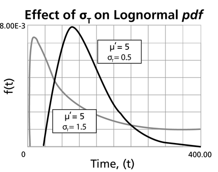
- The degree of skewness increases as [math]\displaystyle{ {{\sigma'}}\,\! }[/math] increases, for a given [math]\displaystyle{ \mu'\,\! }[/math]
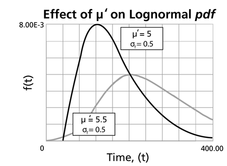
- For the same [math]\displaystyle{ {{\sigma'}}\,\! }[/math], the pdf 's skewness increases as [math]\displaystyle{ {\mu }'\,\! }[/math] increases.
- For [math]\displaystyle{ {{\sigma' }}\,\! }[/math] values significantly greater than 1, the pdf rises very sharply in the beginning, (i.e., for very small values of [math]\displaystyle{ T\,\! }[/math] near zero), and essentially follows the ordinate axis, peaks out early, and then decreases sharply like an exponential pdf or a Weibull pdf with [math]\displaystyle{ 0\lt \beta \lt 1\,\! }[/math].
- The parameter, [math]\displaystyle{ {\mu }'\,\! }[/math], in terms of the logarithm of the [math]\displaystyle{ {T}'s\,\! }[/math] is also the scale parameter, and not the location parameter as in the case of the normal pdf.
- The parameter [math]\displaystyle{ {{\sigma'}}\,\! }[/math], or the standard deviation of the [math]\displaystyle{ {T}'s\,\! }[/math] in terms of their logarithm or of their [math]\displaystyle{ {T}'\,\! }[/math], is also the shape parameter and not the scale parameter, as in the normal pdf, and assumes only positive values.
Lognormal Distribution Parameters in ReliaSoft's Software
In ReliaSoft's software, the parameters returned for the lognormal distribution are always logarithmic. That is: the parameter [math]\displaystyle{ {\mu }'\,\! }[/math] represents the mean of the natural logarithms of the times-to-failure, while [math]\displaystyle{ {{\sigma' }}\,\! }[/math] represents the standard deviation of these data point logarithms. Specifically, the returned [math]\displaystyle{ {{\sigma' }}\,\! }[/math] is the square root of the variance of the natural logarithms of the data points. Even though the application denotes these values as mean and standard deviation, the user is reminded that these are given as the parameters of the distribution, and are thus the mean and standard deviation of the natural logarithms of the data. The mean value of the times-to-failure, not used as a parameter, as well as the standard deviation can be obtained through the QCP or the Function Wizard.


