Crow Extended Confidence Bounds Example 2
New format available! This reference is now available in a new format that offers faster page load, improved display for calculations and images and more targeted search.
As of January 2024, this Reliawiki page will not continue to be updated. Please update all links and bookmarks to the latest references at RGA examples and RGA reference examples.
This example appears in the Reliability growth reference.
Calculate the 2-sided confidence bounds at the 90% confidence level on the demonstrated, projected and growth potential MTBF for the Test-Fix-Find-Test data in the Crow Extended Test-Fix-Find-Test Example.
Solution
For this example, there are A, BC and BD failure modes, so the estimated demonstrated failure intensity, [math]\displaystyle{ {{\hat{\lambda }}_{D}}(T)\,\! }[/math], is simply the Crow-AMSAA model applied to all A, BC, and BD data.
- [math]\displaystyle{ {{\hat{\lambda }}_{D}}(T)={{\widehat{\lambda }}_{CA}}=\widehat{\lambda }\widehat{\beta }{{T}^{\widehat{\beta }-1}}=0.12744\,\! }[/math]
Therefore, the demonstrated MTBF is:
- [math]\displaystyle{ MTB{{F}_{D}}={{[{{\hat{\lambda }}_{D}}(T)]}^{-1}}=7.84708\,\! }[/math]
Based on this value, the Fisher Matrix confidence bounds for the demonstrated failure intensity at the 90% confidence level are:
- [math]\displaystyle{ \begin{align} {{[{{\lambda }_{D}}(T)]}_{L}} = & {{{\hat{\lambda }}}_{CA}}(T){{e}^{{{z}_{\alpha }}\sqrt{Var({{{\hat{\lambda }}}_{CA}}(T))}/{{{\hat{\lambda }}}_{CA}}(T)}} \\ = & 0.09339 \end{align}\,\! }[/math]
- [math]\displaystyle{ \begin{align} {{[{{\lambda }_{D}}(T)]}_{U}} = & {{{\hat{\lambda }}}_{CA}}(T){{e}^{-{{z}_{\alpha }}\sqrt{Var({{{\hat{\lambda }}}_{CA}}(T))}/{{{\hat{\lambda }}}_{CA}}(T)}} \\ = & 0.17390 \end{align}\,\! }[/math]
The Fisher Matrix confidence bounds for the demonstrated MTBF at the 90% confidence level are:
- [math]\displaystyle{ \begin{align} MTB{{F}_{{{D}_{L}}}} = & \frac{1}{{{[{{\lambda }_{D}}(T)]}_{U}}} \\ = & 5.75054 \\ MTB{{F}_{{{D}_{U}}}} = & \frac{1}{{{[{{\lambda }_{D}}(T)]}_{L}}} \\ = & 10.70799 \end{align}\,\! }[/math]
The Crow confidence bounds for the demonstrated MTBF at the 90% confidence level are:
- [math]\displaystyle{ \begin{align} MTB{{F}_{{{D}_{L}}}} = & \frac{1}{{{[{{\lambda }_{D}}(T)]}_{U}}} \\ = & \frac{1}{{{\widehat{\lambda }}_{D}}(T)\tfrac{{{\chi }^{2}}(2N,\alpha /2)}{2N}} \\ = & 5.6325 \\ MTB{{F}_{{{D}_{U}}}} = & \frac{1}{{{[{{\lambda }_{D}}(T)]}_{L}}} \\ = & \frac{1}{{{\widehat{\lambda }}_{D}}(T)\tfrac{{{\chi }^{2}}(2N,1-\alpha /2)}{2N}} \\ = & 10.8779 \end{align}\,\! }[/math]
The projected failure intensity is:
- [math]\displaystyle{ \begin{align} \hat{\lambda}_P (T) &= \widehat{\lambda}_{CA} - \widehat{\lambda}_{BD} + \sum_{i=1}^M (1-d_i) \tfrac{N_i}{T} + \bar{d}\widehat{h}(T|BD) \\ &= 0.0885 \,\! \end{align} }[/math]
Based on this value, the Fisher Matrix confidence bounds at the 90% confidence level for the projected failure intensity are:
- [math]\displaystyle{ \begin{align} {{[{{\lambda }_{P}}(T)]}_{L}} = & {{{\hat{\lambda }}}_{P}}(T){{e}^{{{z}_{\alpha }}\sqrt{Var({{{\hat{\lambda }}}_{P}}(T))}/{{{\hat{\lambda }}}_{P}}(T)}} \\ = & 0.0681 \end{align}\,\! }[/math]
- [math]\displaystyle{ \begin{align} {{[{{\lambda }_{P}}(T)]}_{U}} = & {{{\hat{\lambda }}}_{P}}(T){{e}^{-{{z}_{\alpha }}\sqrt{Var({{{\hat{\lambda }}}_{P}}(T))}/{{{\hat{\lambda }}}_{P}}(T)}} \\ = & 0.1152 \end{align}\,\! }[/math]
The Fisher Matrix confidence bounds for the projected MTBF at the 90% confidence level are:
- [math]\displaystyle{ \begin{align} MTB{{F}_{{{P}_{L}}}} = & \frac{1}{{{[{{\lambda }_{P}}(T)]}_{U}}} \\ = & 8.6818 \\ MTB{{F}_{{{P}_{U}}}} = & \frac{1}{{{[{{\lambda }_{P}}(T)]}_{L}}} \\ = & 14.6926 \end{align}\,\! }[/math]
The Crow confidence bounds for the projected failure intensity are:
- [math]\displaystyle{ \begin{align} {{[{{\lambda }_{P}}(T)]}_{L}} = & {{{\hat{\lambda }}}_{P}}(T)+\frac{{{C}^{2}}}{2}-\sqrt{{{{\hat{\lambda }}}_{P}}(T)\cdot \ \,{{C}^{2}}+\frac{{{C}^{4}}}{4}} \\ = & 0.0672 \\ {{[{{\lambda }_{P}}(T)]}_{U}} = & {{{\hat{\lambda }}}_{P}}(T)+\frac{{{C}^{2}}}{2}+\sqrt{{{{\hat{\lambda }}}_{P}}(T)\cdot {{C}^{2}}+\frac{{{C}^{4}}}{4}} \\ = & 0.1166 \end{align}\,\! }[/math]
The Crow confidence bounds for the projected MTBF at the 90% confidence level are:
- [math]\displaystyle{ \begin{align} MTB{{F}_{{{P}_{L}}}} = & \frac{1}{{{[{{\widehat{\lambda }}_{P}}(T)]}_{U}}} \\ = & 8.5743 \\ MTB{{F}_{{{P}_{U}}}} = & \frac{1}{{{[{{\widehat{\lambda }}_{P}}(T)]}_{L}}} \\ = & 14.8769 \end{align}\,\! }[/math]
The growth potential failure intensity is:
- [math]\displaystyle{ \widehat{\lambda}_{GP} = \widehat{\lambda}_{CA} - \widehat{\lambda}_{BD} + \sum_{i=1}^M (1-d_i) \tfrac{N_i}{T} = 0.0670 \,\! }[/math]
Based on this value, the Fisher Matrix and Crow confidence bounds at the 90% confidence level for the growth potential failure intensity are:
- [math]\displaystyle{ \begin{align} {{r}_{L}} = & {{{\hat{r}}}_{GP}}+\frac{{{C}^{2}}}{2}-\sqrt{{{{\hat{r}}}_{GP}}{{C}^{2}}+\frac{{{C}^{4}}}{4}} \\ = & 0.0488 \\ {{r}_{U}} = & {{{\hat{r}}}_{GP}}+\frac{{{C}^{2}}}{2}+\sqrt{{{{\hat{r}}}_{GP}}{{C}^{2}}+\frac{{{C}^{4}}}{4}} \\ = & 0.0919 \end{align}\,\! }[/math]
The Fisher Matrix and Crow confidence bounds for the growth potential MTBF at the 90% confidence level are:
- [math]\displaystyle{ \begin{align} MTB{{F}_{G{{P}_{L}}}} = & \frac{1}{{{r}_{U}}} \\ = & 10.8790 \\ MTB{{F}_{G{{P}_{U}}}} = & \frac{1}{{{r}_{L}}} \\ = & 20.4855 \end{align}\,\! }[/math]
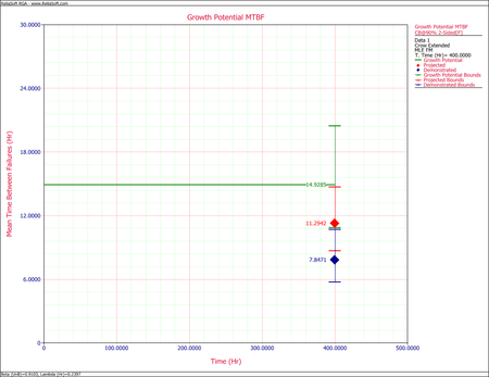
The figure below shows the Fisher Matrix confidence bounds at the 90% confidence level for the demonstrated, projected and growth potential MTBF.
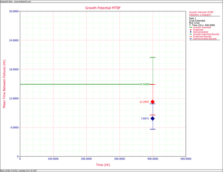
The next figure shows these bounds based on the Crow method.


