Appendix B: Parameter Estimation

This appendix presents two methods for estimating the parameters of accelerated life test data analysis models (ALTA models). The graphical method, which is based on probability plotting or least squares (Rank Regression on X or Rank Regression on Y), has some limitations. Therefore, the Maximum Likelihood Estimation (MLE) method is used for all parameter estimation in ALTA.

Graphical Method

The graphical method for estimating the parameters of accelerated life data involves generating two types of plots. First, the life data at each individual stress level are plotted on a probability paper appropriate to the assumed life distribution (i.e., Weibull, exponential, or lognormal). This can be done using either Probability Plotting or Least Squares (Rank Regression).

The parameters of the distribution at each stress level are then estimated from the plot. Once these parameters have been estimated at each stress level, the second plot is created on a paper that linearizes the assumed life-stress relationship (e.g., Arrhenius, inverse power law, etc.). To do this, a life characteristic must be chosen to be plotted. The life characteristic can be any percentile, such as B(x) life, the scale parameter, mean life, etc. The plotting paper used is a special type of paper that linearizes the life-stress relationship. For example, a log-log paper linearizes the inverse power law relationship, and a log-reciprocal paper linearizes the Arrhenius relationship. The parameters of the model are then estimated by solving for the slope and the intercept of the line.

Example of Graphical Method for Accelerated Life Data

Consider the following times-to-failure data at three different stress levels.

Stress	393 psi	408 psi	423 psi
Time Failed (hrs)	3450	3300	2645
	4340	3720	3100
	4760	4180	3400
	5320	4560	3800
	5740	4920	4100
	6160	5280	4400
	6580	5640	4700
	7140	6233	5100
	8101	6840	5700
	8960	7380	6400

Estimate the parameters for a Weibull assumed life distribution and for the inverse power law life-stress relationship.

Solution

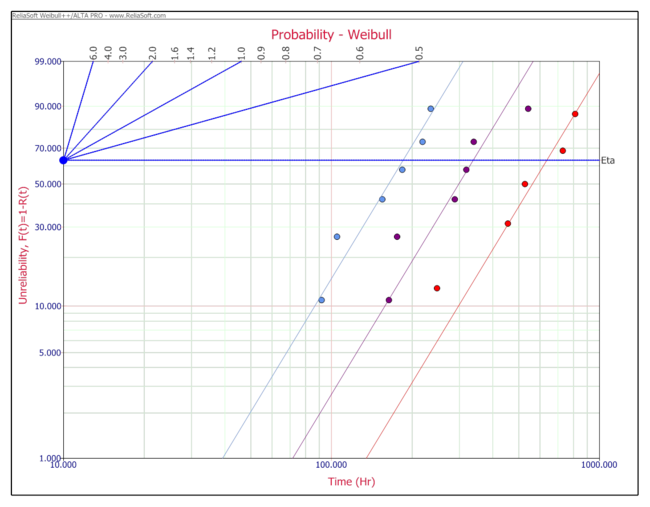
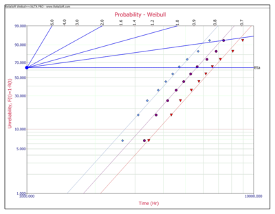
First the parameters of the Weibull distribution need to be determined. The data are individually analyzed (for each stress level) using the probability plotting method, or software such as ReliaSoft's Weibull++, with the following results:

[math]\displaystyle{ \begin{align} & [{{\widehat{\beta }}_{1}}= & 3.8,\text{ }{{\widehat{\eta }}_{1}}=6692] \\ & \text{ }\!\![\!\!\text{ }{{\widehat{\beta }}_{2}}= & 4.2,\text{ }{{\widehat{\eta }}_{2}}=5716] \\ & [{{\widehat{\beta }}_{3}}= & 4,\text{ }{{\widehat{\eta }}_{3}}=4774] \end{align} }[/math]

where:
• [math]\displaystyle{ {{\widehat{\beta }}_{1}}, }[/math] [math]\displaystyle{ {{\widehat{\eta }}_{1}} }[/math] are the parameters of the 393 psi data.

• [math]\displaystyle{ {{\widehat{\beta }}_{2}}, }[/math] [math]\displaystyle{ {{\widehat{\eta }}_{2}} }[/math] are the parameters of the 408 psi data.

• [math]\displaystyle{ {{\widehat{\beta }}_{3}}, }[/math] [math]\displaystyle{ {{\widehat{\eta }}_{3}} }[/math] are the parameters of the 423 psi data.

Since the shape parameter, [math]\displaystyle{ \beta , }[/math] is not common for the three stress levels, the average value is estimated.

[math]\displaystyle{ {{\widehat{\beta }}_{common}}=4 }[/math]

Averaging the betas is one of many simple approaches available. One can also use a weighted average, since the uncertainty on beta is greater for smaller sample sizes. In most practical applications the value of [math]\displaystyle{ \widehat{\beta } }[/math] will vary (even though it is assumed constant) due to sampling error, etc. The variability in the value of [math]\displaystyle{ \widehat{\beta } }[/math] is a source of error when performing analysis by averaging the betas. MLE analysis, which uses a common [math]\displaystyle{ \widehat{\beta } }[/math] , is not susceptible to this error. MLE analysis is the method of parameter estimation used in ALTA and it is explained in the next section.

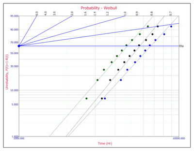
Redraw each line with a [math]\displaystyle{ \widehat{\beta }=4, }[/math] and estimate the new etas, as follows:

[math]\displaystyle{ \begin{align} & {{\widehat{\eta }}_{1}}= & 6650 \\ & {{\widehat{\eta }}_{2}}= & 5745 \\ & {{\widehat{\eta }}_{3}}= & 4774 \end{align} }[/math]

The IPL relationship is given by:

[math]\displaystyle{ L(V)=\frac{1}{K{{V}^{n}}} }[/math]

where:
[math]\displaystyle{ L }[/math] represents a quantifiable life measure ( eta in the Weibull case), [math]\displaystyle{ V }[/math] represents the stress level, [math]\displaystyle{ K }[/math] is one of the parameters, and [math]\displaystyle{ n }[/math] is another model parameter. The relationship is linearized by taking the logarithm of both sides which yields:

[math]\displaystyle{ \ln (L)=-\ln K-n\ln V }[/math]

where [math]\displaystyle{ L=\eta }[/math] , (- [math]\displaystyle{ \ln K) }[/math] is the intercept, and (- [math]\displaystyle{ n) }[/math] is the slope of the line.

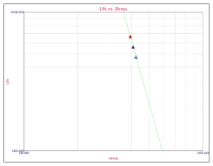
The values of eta obtained previously are now plotted on a log-linear scale yielding the following plot:

The slope of the line is the [math]\displaystyle{ n }[/math] parameter, which is obtained from the plot:

[math]\displaystyle{ \begin{align} & Slope=\ \frac{\ln ({{T}_{2}})-\ln ({{T}_{1}})}{\ln ({{V}_{2}})-\ln ({{V}_{1}})} =\ \frac{\ln (10,000)-\ln (6,000)}{\ln (360)-\ln (403)} =\ -4.5272 \end{align} }[/math]

Thus:

[math]\displaystyle{ \widehat{n}=4.5272 }[/math]

Solving the inverse power law equation with respect to [math]\displaystyle{ K }[/math] yields:

[math]\displaystyle{ \widehat{K}=\frac{1}{L{{V}^{n}}} }[/math]

Substituting V=403, the corresponding L (from the plot), L=6,000 and the previously estimated [math]\displaystyle{ n\ \ : }[/math]

[math]\displaystyle{ \begin{align} & \widehat{K}=\ \frac{1}{6000\text{ }{{403}^{4.5272}}} =\ 2.67\cdot {{10}^{-16}} \end{align} }[/math]

Comments on the Graphical Method

Although the graphical method is simple, it is quite laborious. Furthermore, many issues surrounding its use require careful consideration. Some of these issues are presented next:

• What happens when no failures are observed at one or more stress level? In this case, plotting methods cannot be employed. Discarding the data would be a mistake since every piece of life data information is important.

• In the step at which the life-stress relationship is linearized and plotted to obtain its parameters, you must be able to linearize the function, which is not always possible.

• In real accelerated tests the data sets are small. Separating them and individually plotting them, and then subsequently replotting the results, increases the underlying error.

• During initial parameter estimation, the parameter that is assumed constant will more than likely vary. What value do you use?

• Confidence intervals on all of the results cannot be ascertained using graphical methods.

The maximum likelihood estimation parameter estimation method described next overcomes these shortfalls, and is the method utilized in ALTA.

Maximum Likelihood Estimation (MLE) Method

The idea behind maximum likelihood parameter estimation is to determine the parameters that maximize the probability (likelihood) of the sample data. From a statistical point of view, the method of maximum likelihood is considered to be more robust (with some exceptions) and yields estimators with good statistical properties. In other words, MLE methods are versatile and apply to most models and to different types of data. In addition, they provide efficient methods for quantifying uncertainty through confidence bounds. For a detailed discussion of this analysis method for a single life distribution, see Maximum Likelihood Estimation.

MLE of Accelerated Life Data

The maximum likelihood solution for accelerated life test data is formulated in the same way as described in Maximum Likelihood Estimation for a single life distribution. However, in this case, the stress level of each individual observation is included in the likelihood function. Consider a continuous random variable [math]\displaystyle{ x(v), }[/math] where [math]\displaystyle{ v }[/math] is the stress. The [math]\displaystyle{ pdf }[/math] of the random variable now becomes a function of both [math]\displaystyle{ x }[/math] and [math]\displaystyle{ v }[/math] :

[math]\displaystyle{ f(x,v;{{\theta }_{1}},{{\theta }_{2}},...,{{\theta }_{k}}) }[/math]

where [math]\displaystyle{ {{\theta }_{1}},{{\theta }_{2}},...,{{\theta }_{k}} }[/math] are [math]\displaystyle{ k }[/math] unknown constant parameters which need to be estimated. Conduct an experiment and obtain [math]\displaystyle{ N }[/math] independent observations, [math]\displaystyle{ {{x}_{1}},{{x}_{2}},...,{{x}_{N}} }[/math] each at a corresponding stress, [math]\displaystyle{ {{v}_{1}}, }[/math] [math]\displaystyle{ {{v}_{2}},..., }[/math] [math]\displaystyle{ {{v}_{N}} }[/math] . Then the likelihood function for complete data is given by:

[math]\displaystyle{ L(({{x}_{1}},\text{ }{{v}_{1}}),({{x}_{2}},\text{ }{{v}_{2}}),...,({{x}_{N}},\text{ }{{v}_{N}})|{{\theta }_{1}},{{\theta }_{2}},...,{{\theta }_{k}})=\underset{i=1}{\overset{N}{\mathop \prod }}\,f({{x}_{i}},{{v}_{i}};{{\theta }_{1}},{{\theta }_{2}},...,{{\theta }_{k}}) }[/math]

[math]\displaystyle{ i=1,2,...,N }[/math]

The logarithmic likelihood function is given by:

[math]\displaystyle{ \Lambda =\ln L=\underset{i=1}{\overset{N}{\mathop \sum }}\,\ln f({{x}_{i}},{{v}_{i}};{{\theta }_{1}},{{\theta }_{2}},...,{{\theta }_{k}}) }[/math]

The maximum likelihood estimators (MLE) of [math]\displaystyle{ {{\theta }_{1}},{{\theta }_{2}},...,{{\theta }_{k}}, }[/math] are obtained by maximizing [math]\displaystyle{ L }[/math] or [math]\displaystyle{ \Lambda . }[/math]

In this case, [math]\displaystyle{ {{\theta }_{1}},{{\theta }_{2}},...,{{\theta }_{k}} }[/math] are the parameters of the combined model which includes the parameters of the life distribution and the parameters of the life-stress relationship. Note that in the above equations, [math]\displaystyle{ N }[/math] is the total number of observations. This means that the sample size is no longer broken into the number of observations at each stress level. In Example 1, the sample size at the stress level of 20V was 4, and 15 at 36V. Using the above equations, however, the test's sample size is 19.

Once the parameters are estimated, they can be substituted back into the life distribution and the life-stress relationship.

Example of MLE for Accelerated Life Data

The following example illustrates the use of the MLE method on accelerated life test data. Consider the inverse power law relationship, given by:

[math]\displaystyle{ L(V)=\frac{1}{K{{V}^{n}}} }[/math]

where [math]\displaystyle{ L }[/math] represents a quantifiable life measure, [math]\displaystyle{ V }[/math] represents the stress level, [math]\displaystyle{ K }[/math] is one of the parameters, and [math]\displaystyle{ n }[/math] is another model parameter. Assume that the life at each stress follows a Weibull distribution, with a [math]\displaystyle{ pdf }[/math] given by:

[math]\displaystyle{ f(t)=\frac{\beta }{\eta }{{\left( \frac{T}{\eta } \right)}^{\beta -1}}{{e}^{-{{\left( \tfrac{T}{\eta } \right)}^{\beta }}}} }[/math]

where the time-to-failure, [math]\displaystyle{ t }[/math] , is a function of stress, [math]\displaystyle{ V }[/math] .

A common life measure needs to determined so that it can be easily included in the Weibull [math]\displaystyle{ pdf }[/math]. In this case, setting [math]\displaystyle{ \eta =L(V) }[/math] (which is the life at 63.2%) and substituting in the Weibull [math]\displaystyle{ pdf }[/math], yields the following IPL-Weibull [math]\displaystyle{ pdf }[/math] :

[math]\displaystyle{ f(t,V)=\beta K{{V}^{n}}{{\left( K{{V}^{n}}T \right)}^{\beta -1}}{{e}^{-{{\left( K{{V}^{n}}T \right)}^{\beta }}}} }[/math]

The log-likelihood function for the complete data is given by:

Note that [math]\displaystyle{ \beta }[/math] is now the common shape parameter to solve for, along with [math]\displaystyle{ K }[/math] and [math]\displaystyle{ n. }[/math]

Conclusions

In this appendix, two methods for estimating the parameters of accelerated life testing models were presented. First, the graphical method was illustrated using a probability plotting method for obtaining the parameters of the life distribution. The parameters of the life-stress relationship were then estimated graphically by linearizing the model. However, not all life-stress relationships can be linearized. In addition, estimating the parameters of each individual distribution leads to an accumulation of uncertainties, depending on the number of failures and suspensions observed at each stress level. Furthermore, the slopes (shape parameters) of each individual distribution are rarely equal (common). Using the graphical method, one must estimate a common shape parameter (usually the average) and repeat the analysis. By doing so, further uncertainties are introduced on the estimates, and these are uncertainties that cannot be quantified. The second method, the Maximum Likelihood Estimation, treated both the life distribution and the life-stress relationship as one model, the parameters of that model can be estimated using the complete likelihood function. Doing so, a common shape parameter is estimated for the model, thus eliminating the uncertainties of averaging the individual shape parameters. All uncertainties are accounted for in the form of confidence bounds (presented in detail in Appendix D), which are quantifiable because they are obtained based on the overall model.