Warranty Data Analysis

The Warranty Analysis Folio in Weibull++ provides three different data entry formats for warranty data. It also allows the user to automatically perform a life data analysis on this type of data, allows the prediction of future failures through the use of conditional probability analysis and provides methods for detecting outliers.

Warranty Data Entry Types

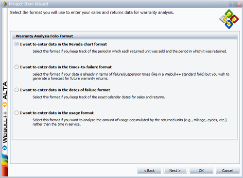
Weibull++ allows for data entry utilizing four common formats for storing sales and returns information. Specifically:

1) Nevada Chart Format

2) Time-to-Failure Format

3) Dates of Failure Format

4) Usage Format

These formats are explained in the next sections.

Nevada Chart Format

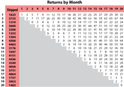
Field information frequently appears in terms of units produced and/or shipped in a certain time period, with the resulting returns for that production lot in the subsequent time periods. This information can be arranged in a diagonal chart, as displayed in the following figure.

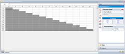
In Weibull++ this window is as shown next:

Time-to-Failure Format

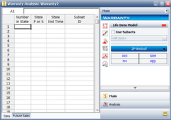
This format is similar to the Standard Folio data entry format (all number of units, failure times and suspension times are entered by the user), as discussed previously. The difference is that when the data is used within the context of warranty analysis, the automatic ability to generate forecasts is available to the user. In Weibull++ this window is as shown next:

Dates of Failure Format

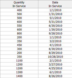
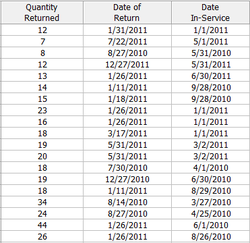
Another common way for reporting field information is to enter a date and quantity of sales or shipments, Quantity In-Service Data, and the date and quantity of returns, Quantity Returned Data, as illustrated in the following tables.

Quality In-Service Data

Quantity Returned Data

Note that in order to identify which lot the unit comes from, a failure is identified by a return date and the date of when it was put in service. The date that the unit went into service is then associated with the lot going into service during that time period. Lots can be used with the optional ID column which is covered in the sections that follow.

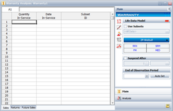
In Weibull++ this window is as shown next:

[math]\displaystyle{ }[/math]

Usage Format

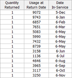
Often the driving factor for reliability is usage rather than time. For example, in the automotive industry, the failure behavior in the majority of the products is mileage-dependent rather than time-dependent. This format allows specifying Quantity In-Service Data, and the usage at return date and Quantity Return Data, as illustrated in the following tables.

Quality In-Service Data

Note that, like in the dates of failure format, in order to identify which lot the unit comes from, a failure is identified by the return number and the date of when it was put in service. The date that the returned unit went into service associates the returned unit with the lot it belonged to when it started operation. However, the return data is in terms of usage and not date of return. Therefore the usage of the units needs to be specified as a constant usage per unit time or as a distribution. This allows determining the expected usage of the surviving units (See Example 2).

Warranty Analysis (Nevada Format)

The Nevada Format allows the user to convert shipping and warranty return data into the standard reliability data form of failures and suspensions so that it can easily be analyzed with traditional life data analysis methods. For each time period in which a number of products are shipped, there will be a certain number of returns or failures in subsequent time periods, while the rest of the population that was shipped will continue to operate in the following time periods. For example, if 500 units are shipped in May, and 10 of those units are warranty returns in June, that is equivalent to 10 failures at a time of one month. The other 450 units will go on to operate and possibly fail in months that follow. At the end of the analysis period, all of the units that were shipped and have not failed in the time since shipment are considered to be suspensions. This process is repeated for each shipment and the results tabulated for each particular failure and suspension time prior to reliability analysis. This process may sound confusing, but it is actually just a matter of careful bookkeeping, and is illustrated with the example that follows.

Example 1:

The Warranty Analysis Folio in Weibull++ provides three different data entry formats for warranty data. It also allows the user to automatically perform a life data analysis on this type of data, allows the prediction of future failures through the use of conditional probability analysis and provides methods for detecting outliers.

Warranty Data Entry Types

Weibull++ allows for data entry utilizing four common formats for storing sales and returns information. Specifically:

1) Nevada Chart Format

2) Time-to-Failure Format

3) Dates of Failure Format

4) Usage Format

These formats are explained in the next sections.

Nevada Chart Format

Field information frequently appears in terms of units produced and/or shipped in a certain time period, with the resulting returns for that production lot in the subsequent time periods. This information can be arranged in a diagonal chart, as displayed in the following figure.

In Weibull++ this window is as shown next:

Time-to-Failure Format

This format is similar to the Standard Folio data entry format (all number of units, failure times and suspension times are entered by the user), as discussed previously. The difference is that when the data is used within the context of warranty analysis, the automatic ability to generate forecasts is available to the user. In Weibull++ this window is as shown next:

Dates of Failure Format

Another common way for reporting field information is to enter a date and quantity of sales or shipments, Quantity In-Service Data, and the date and quantity of returns, Quantity Returned Data, as illustrated in the following tables.

Quality In-Service Data

Quantity Returned Data

Note that in order to identify which lot the unit comes from, a failure is identified by a return date and the date of when it was put in service. The date that the unit went into service is then associated with the lot going into service during that time period. Lots can be used with the optional ID column which is covered in the sections that follow.

In Weibull++ this window is as shown next:

[math]\displaystyle{ }[/math]

Usage Format

Often the driving factor for reliability is usage rather than time. For example, in the automotive industry, the failure behavior in the majority of the products is mileage-dependent rather than time-dependent. This format allows specifying Quantity In-Service Data, and the usage at return date and Quantity Return Data, as illustrated in the following tables.

Quality In-Service Data

Note that, like in the dates of failure format, in order to identify which lot the unit comes from, a failure is identified by the return number and the date of when it was put in service. The date that the returned unit went into service associates the returned unit with the lot it belonged to when it started operation. However, the return data is in terms of usage and not date of return. Therefore the usage of the units needs to be specified as a constant usage per unit time or as a distribution. This allows determining the expected usage of the surviving units (See Example 2).

Warranty Analysis (Nevada Format)

The Nevada Format allows the user to convert shipping and warranty return data into the standard reliability data form of failures and suspensions so that it can easily be analyzed with traditional life data analysis methods. For each time period in which a number of products are shipped, there will be a certain number of returns or failures in subsequent time periods, while the rest of the population that was shipped will continue to operate in the following time periods. For example, if 500 units are shipped in May, and 10 of those units are warranty returns in June, that is equivalent to 10 failures at a time of one month. The other 450 units will go on to operate and possibly fail in months that follow. At the end of the analysis period, all of the units that were shipped and have not failed in the time since shipment are considered to be suspensions. This process is repeated for each shipment and the results tabulated for each particular failure and suspension time prior to reliability analysis. This process may sound confusing, but it is actually just a matter of careful bookkeeping, and is illustrated with the example that follows.

Example 1:

Warranty Analysis (Usage Format)

Warranty data analysis relies on the estimation of a failure distribution based on data including the number of returns and the number of surviving units in the field and the age associated with those units. The Usage Format allows the user to convert shipping and warranty return data into the standard reliability data for of failures and suspensions when the return information is based on usage rather than return dates or periods.

Suppose that you have been collecting sales (units in service) and returns data. For the returns data, you can determine the number of failures and their usage (by reading the odometer value, for example). Determining the number of surviving units (suspensions) and their ages is a straightforward step. By taking the difference between the analysis date and the date when a unit was put in service, you can determine the age of the surviving units.

What is unknown, however, is the exact usage accumulated by each surviving unit. The key part of the usage-based warranty analysis is the determination of the usage of the surviving units based on their age. Therefore, the analyst needs to have an idea about the usage of the product. This can be obtained, for example, from customer surveys or by designing the products to collect usage data. For example, in automotive applications, engineers often use 12,000 miles/year as an average usage. Based on this average, the usage of an item that has been in the field for 6 months and has not yet failed would be 6,000 miles. So to obtain the usage of a suspension based on an average usage, one could take the time of each suspension and multiply it by this average usage. As you see, in this situation the analysis becomes straightforward. With the usage values and the quantities of the returned units, a failure distribution can be constructed and subsequent warranty analysis becomes possible.

Alternatively, and more realistically, instead of using an average usage, an actual distribution that reflects the variation in usage and customer behavior can be used. This distribution describes the usage of a unit over a certain time period (e.g. 1 year, 1 month, etc). This probabilistic model can be used to estimate the usage for all surviving components in service and the percentage of users running the product at different usage rates. In the automotive example, for instance, such a distribution can be used to calculate the percentage of customers that drive 0-200 miles/month, 200-400 miles/month, etc. We can take these percentages and multiply them by the number of suspensions to find the number of items that have been accumulating usage values in these ranges.

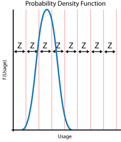
To proceed with applying a usage distribution, the usage distribution is divided into increments based on a specified interval width denoted as [math]\displaystyle{ Z }[/math] . The usage distribution, [math]\displaystyle{ Q }[/math] , is divided into intervals of [math]\displaystyle{ 0+Z }[/math] , [math]\displaystyle{ Z+Z }[/math] , [math]\displaystyle{ 2Z+Z }[/math] , etc., or [math]\displaystyle{ {{x}_{i}}={{x}_{i-1}}+Z }[/math] , as shown in the next figure.

The interval width should be selected such that it creates segments that are large enough to contain adequate numbers of suspensions within the intervals.

The percentage of suspensions that belong to each usage interval is calculated as follows:

[math]\displaystyle{ F({{x}_{i}})=Q({{x}_{i}})-Q({{x}_{i}}-1) }[/math]

where:

[math]\displaystyle{ Q() }[/math] is the usage distribution Cumulative Density Function, [math]\displaystyle{ cdf }[/math] .

[math]\displaystyle{ x }[/math] represents the intervals used in apportioning the suspended population.

We also define a suspension group as a collection of suspensions that have the same age.

The above percentage of suspensions can be translated to numbers of suspensions within each interval, [math]\displaystyle{ {{x}_{i}} }[/math] . This is done by taking each group of suspensions and multiplying it by each [math]\displaystyle{ F({{x}_{i}}) }[/math] , or:

[math]\displaystyle{ \begin{align} & {{N}_{1,j}}= & F({{x}_{1}})\times N{{S}_{j}} \\ & {{N}_{2,j}}= & F({{x}_{2}})\times N{{S}_{j}} \\ & & ... \\ & {{N}_{n,j}}= & F({{x}_{n}})\times N{{S}_{j}} \end{align} }[/math]

where:

[math]\displaystyle{ {{N}_{n,j}} }[/math] is the number of suspensions that belong to each interval.

[math]\displaystyle{ N{{S}_{j}} }[/math] is the jth group of suspensions from the data set.

This is repeated for all the groups of suspensions.

The age of the suspensions is calculated by subtracting the Date In-Service ( [math]\displaystyle{ DIS }[/math] ), the date at which the unit started operation, from the calculation End Date ( [math]\displaystyle{ ED }[/math] ). This is the Time In-Service ( [math]\displaystyle{ TIS }[/math] ) value that describes the age of the surviving unit.

[math]\displaystyle{ TIS=ED-DIS }[/math]

Note: [math]\displaystyle{ TIS }[/math] is in the same time units as the period in which the usage distribution is defined.

For each [math]\displaystyle{ {{N}_{k,j}} }[/math] , the usage is calculated as:

[math]\displaystyle{ Uk,j=xi\times TISj }[/math]

After this step, the usage of each suspension group is estimated. The data can be combined with the failures and a failure distribution can be fitted.

Example 2: Warranty Analysis Usage Format Example

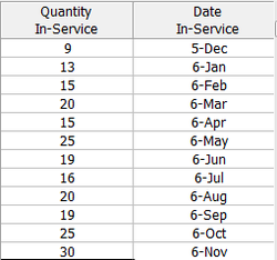
Suppose that an automotive manufacturer collects the warranty returns and sales data given in the following tables. Convert this information to life data and analyze it using the lognormal distribution.

Quality In-Service Data

Quantity In-Service	Date In-Service
9	Dec-09
13	Jan-10
15	Feb-10
20	Mar-10
15	Apr-10
25	May-10
19	Jun-10
16	Jul-10
20	Aug-10
19	Sep-10
25	Oct-10
30	Nov-10

Quality Return Data

Quantity Returned	Usage at Return Date	Date In-Service
1	9072	Dec-09
1	9743	Jan-10
1	6857	Feb-10
1	7651	Mar-10
1	5083	May-10
1	5990	May-10
1	7432	May-10
1	8739	May-10
1	3158	Jun-10
1	1136	Jul-10
1	4646	Aug-10
1	3965	Sep-10
1	3117	Oct-10
1	3250	Nov-10

Solution

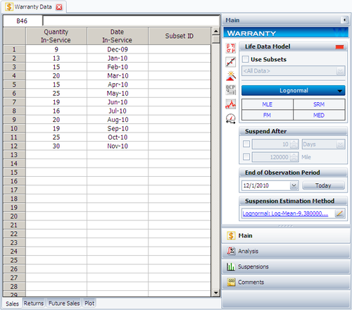
Create a warranty analysis folio and select the usage format. Enter the data from the tables in the Sales, Returns and Future Sales sheets. The warranty data were collected until 12/1/2010; therefore, on the control panel, set the End of Observation Period to that date. Set the failure distribution to Lognormal, as shown next.

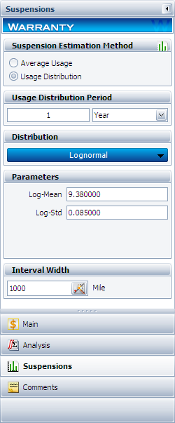
In this example, the manufacturer has been documenting the mileage accumulation per year for this type of product across the customer base in comparable regions for many years. The yearly usage has been determined to follow a lognormal distribution with [math]\displaystyle{ {{\mu }_{T\prime }}=9.38\,\! }[/math], [math]\displaystyle{ {{\sigma }_{T\prime }}=0.085\,\! }[/math]. The Interval Width is defined to be 1,000 miles. Enter the information about the usage distribution on the Suspensions page of the control panel, as shown next.

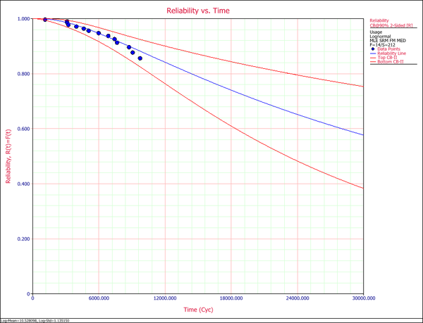
Click Calculate to analyze the data set. The parameters are estimated to be:

[math]\displaystyle{ \begin{align} & {{\mu }_{T\prime }}= & 10.528098 \\ & {{\sigma }_{T\prime }}= & 1.135150 \end{align}\,\! }[/math]

The reliability plot (with mileage being the random variable driving reliability), along with the 90% confidence bounds on reliability, is shown next.

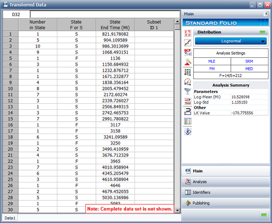
In this example, the life data set contains 14 failures and 212 suspensions spread according to the defined usage distribution. You can display this data in a standard folio by choosing Warranty > Transfer Life Data > Transfer Life Data to New Folio. The failures and suspensions data set, as presented in the standard folio, is shown next (showing only the first 30 rows of data).

Warranty Prediction

Once a life data analysis has been performed on warranty data, this information can be used to predict how many warranty returns there will be in subsequent time periods. This methodology uses the concept of conditional reliability (see Chapter Basic Statistical Background) to calculate the probability of failure for the remaining units for each shipment time period. This conditional probability of failure is then multiplied by the number of units at risk from that particular shipment period that are still in the field (i.e. the suspensions) in order to predict the number of failures or warranty returns expected for this time period. The next example illustrates this.

Example 3:

Analysis of Non-Homogeneous Warranty Data

In the previous sections and examples it is important to note that the underlying assumption was that the population was homogeneous. In other words, all sold and returned units were exactly the same, i.e. the same population with no design changes and/or modifications. In many situations, as the product matures, design changes are made to enhance and/or improve the reliability of the product. Obviously, an improved product will exhibit different failure characteristics than its predecessor. To analyze such cases, where the population is non-homogeneous, one needs to extract each homogenous group, fit a life model to each group and then project the expected returns for each group based on the number of units at risk for each specific group.

Using IDs in Weibull++

Weibull++ uses the optional IDs column to differentiate between product versions or different designs (lots). Based on this entry, the data are then automatically separated and the parameters for each lot computed. Based on the computed parameters, failure projections can then be obtained. Note that it is important to realize that the same limitations as discussed previously, with regards to the number of failures that are needed, are also applicable here. In other words, distributions can be automatically fitted to lots that have return (failure) data, whereas if no returns have been experienced yet (either because the units are going to be introduced in the future or because no failures happened yet), the user will be asked to specify the parameters, since they can not be computed. Consequently, subsequent estimation/predictions related to these lots would be based on the user specified parameters. Following is an example that illustrates the use of IDs.

Example 4: Warranty Analysis Non-Homogeneous Data Example

A company keeps track of its production and returns. The company uses the dates of failure format to record the data. For the product in question, three versions (A, B and C) have been produced and put in service. The in-service data is as follows (using the Month/Day/Year date format):

[math]\displaystyle{ \begin{matrix} Quantity In-Service & Date of In-Service & ID \\ \text{400} & \text{1/1/2005} & \text{Model A} \\ \text{500} & \text{1/31/2005} & \text{Model A} \\ \text{500} & \text{5/1/2005} & \text{Model A} \\ \text{600} & \text{5/31/2005} & \text{Model A} \\ \text{550} & \text{6/30/2005} & \text{Model A} \\ \text{600} & \text{7/30/2005} & \text{Model A} \\ \text{800} & \text{9/28/2005} & \text{Model A} \\ \text{200} & \text{1/1/2005} & \text{Model B} \\ \text{350} & \text{3/2/2005} & \text{Model B} \\ \text{450} & \text{4/1/2005} & \text{Model B} \\ \text{300} & \text{6/30/2005} & \text{Model B} \\ \text{200} & \text{8/29/2005} & \text{Model B} \\ \text{350} & \text{10/28/2005} & \text{Model B} \\ \text{1100} & \text{2/1/2005} & \text{Model C} \\ \text{1200} & \text{3/27/2005} & \text{Model C} \\ \text{1200} & \text{4/25/2005} & \text{Model C} \\ \text{1300} & \text{6/1/2005} & \text{Model C} \\ \text{1400} & \text{8/26/2005} & \text{Model C} \\ \end{matrix}\,\! }[/math]

Furthermore, the following sales are forecast:

[math]\displaystyle{ \begin{matrix} Number & Date & ID \\ \text{400} & \text{6/27/2006} & \text{Model A} \\ \text{500} & \text{8/26/2006} & \text{Model A} \\ \text{550} & \text{10/26/2006} & \text{Model A} \\ \text{1200} & \text{7/25/2006} & \text{Model C} \\ \text{1300} & \text{9/27/2006} & \text{Model C} \\ \text{1250} & \text{11/26/2006} & \text{Model C} \\ \end{matrix}\,\! }[/math]

The return data are as follows. Note that in order to identify which lot each unit comes from, and to be able to compute its time-in-service, each return (failure) includes a return date, the date of when it was put in service and the model ID.

[math]\displaystyle{ \begin{matrix} Quantity Returned & Date of Return & Date In-Service & ID \\ \text{12} & \text{1/31/2005} & \text{1/1/2005} & \text{Model A} \\ \text{11} & \text{4/1/2005} & \text{1/31/2005} & \text{Model A} \\ \text{7} & \text{7/22/2005} & \text{5/1/2005} & \text{Model A} \\ \text{8} & \text{8/27/2005} & \text{5/31/2005} & \text{Model A} \\ \text{12} & \text{12/27/2005} & \text{5/31/2005} & \text{Model A} \\ \text{13} & \text{1/26/2006} & \text{6/30/2005} & \text{Model A} \\ \text{12} & \text{1/26/2006} & \text{7/30/2005} & \text{Model A} \\ \text{14} & \text{1/11/2006} & \text{9/28/2005} & \text{Model A} \\ \text{15} & \text{1/18/2006} & \text{9/28/2005} & \text{Model A} \\ \text{23} & \text{1/26/2005} & \text{1/1/2005} & \text{Model B} \\ \text{16} & \text{1/26/2005} & \text{1/1/2005} & \text{Model B} \\ \text{18} & \text{3/17/2005} & \text{1/1/2005} & \text{Model B} \\ \text{19} & \text{5/31/2005} & \text{3/2/2005} & \text{Model B} \\ \text{20} & \text{5/31/2005} & \text{3/2/2005} & \text{Model B} \\ \text{21} & \text{6/30/2005} & \text{3/2/2005} & \text{Model B} \\ \text{18} & \text{7/30/2005} & \text{4/1/2005} & \text{Model B} \\ \text{19} & \text{12/27/2005} & \text{6/30/2005} & \text{Model B} \\ \text{18} & \text{1/11/2006} & \text{8/29/2005} & \text{Model B} \\ \text{11} & \text{2/7/2006} & \text{10/28/2005} & \text{Model B} \\ \text{34} & \text{8/14/2005} & \text{3/27/2005} & \text{Model C} \\ \text{24} & \text{8/27/2005} & \text{4/25/2005} & \text{Model C} \\ \text{44} & \text{1/26/2006} & \text{6/1/2005} & \text{Model C} \\ \text{26} & \text{1/26/2006} & \text{8/26/2005} & \text{Model C} \\ \end{matrix}\,\! }[/math]

Assuming that the given information is current as of 5/1/2006, analyze the data using the lognormal distribution and MLE analysis method for all models (Model A, Model B, Model C), and provide a return forecast for the next ten months.

Solution

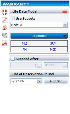
Create a warranty analysis folio and select the dates of failure format. Enter the data from the tables in the Sales, Returns and Future Sales sheets. On the control panel, select the Use Subsets check box, as shown next. This allows the software to separately analyze each subset of data. Use the drop-down list to switch between subset IDs and alter the analysis settings (use the lognormal distribution and MLE analysis method for all models).

In the End of Observation Period field, enter 5/1/2006, and then calculate the parameters. The results are:

[math]\displaystyle{ \begin{matrix} Model A & Model B & Model C \\ \begin{matrix} {{{\hat{\mu }}}^{\prime }}= & \text{11}\text{.28} \\ {{{\hat{\sigma }}}_{T}}= & \text{2}\text{.83} \\ \end{matrix} & \begin{matrix} {{{\hat{\mu }}}^{\prime }}= & \text{8}\text{.11} \\ {{{\hat{\sigma }}}_{T}}= & \text{2}\text{.30} \\ \end{matrix} & \begin{matrix} {{{\hat{\mu }}}^{\prime }}= & \text{9}\text{.79} \\ {{{\hat{\sigma }}}_{T}}= & \text{1}\text{.92} \\ \end{matrix} \\ \end{matrix}\,\! }[/math]

Note that in this example, the same distribution and analysis method were assumed for each of the product models. If desired, different distribution types, analysis methods, confidence bounds methods, etc., can be assumed for each IDs.

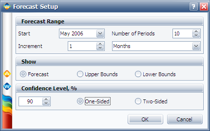
To obtain the expected failures for the next 10 months, click the Generate Forecast icon. In the Forecast Setup window, set the forecast to start on May 2, 2006 and set the number of forecast periods to 10. Set the increment (length of each period) to 1 Month, as shown next.

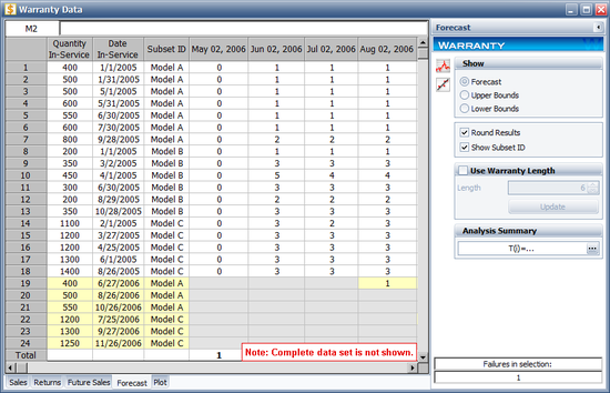
Click OK. A Forecast sheet will be created, with the predicted future returns. The following figure shows part of the Forecast sheet.

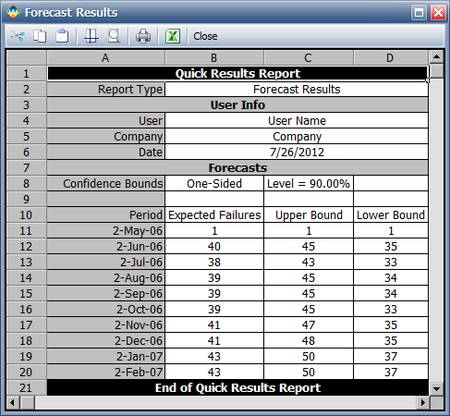
To view a summary of the analysis, click the Show Analysis Summary (...) button. The following figure shows the summary of the forecasted returns.

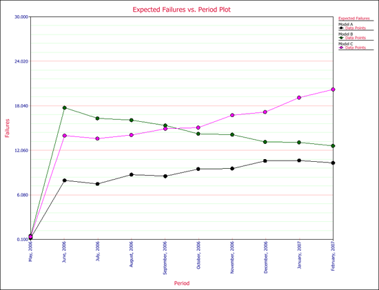
Click the Plot icon and choose the Expected Failures plot. The plot displays the predicted number of returns for each month, as shown next.

Monitoring Warranty Returns Using Statistical Process Control (SPC)

By monitoring and analyzing warranty return data, the user now has the ability to detect specific return periods and/or batches of sales or shipments that may deviate (differ) from the assumed model. This provides the analyst (and the organization) the advantage of early notification of possible deviations in manufacturing, use conditions and/or any other factor that may adversely affect the reliability of the fielded product.

Obviously, the motivation for performing such analysis is to allow for faster intervention to avoid increased costs due to increased warranty returns or more serious repercussions. Additionally, this analysis can also be used to uncover different sub-populations that may exist within this population.

Analysis Method

For each sales period [math]\displaystyle{ i }[/math] and return period [math]\displaystyle{ j }[/math] , the prediction error can be calculated as follows:

[math]\displaystyle{ {{e}_{i,j}}={{\hat{F}}_{i,j}}-{{F}_{i,j}} }[/math]

where [math]\displaystyle{ {{\hat{F}}_{i,j}} }[/math] is the estimated number of failures based on the estimated distribution parameters for the sales period [math]\displaystyle{ i }[/math] and the return period [math]\displaystyle{ j }[/math] , which is calculated using the equation for the conditional probability, and [math]\displaystyle{ {{F}_{i,j}} }[/math] is the actual number of failure for the sales period [math]\displaystyle{ i }[/math] and the return period [math]\displaystyle{ j }[/math] .

Since we are assuming that the model is accurate, [math]\displaystyle{ {{e}_{i,j}} }[/math] should follow a normal distribution with mean value of zero and a standard deviation [math]\displaystyle{ s }[/math] , where:

[math]\displaystyle{ {{\bar{e}}_{i,j}}=\frac{\underset{i}{\mathop{\sum }}\,\underset{j}{\mathop{\sum }}\,{{e}_{i,j}}}{n}=0 }[/math]

and [math]\displaystyle{ n }[/math] is the total number of return data (total number of residuals).

The estimated standard deviation of the prediction errors can then be calculated by:

[math]\displaystyle{ s=\sqrt{\frac{1}{n-1}\underset{i}{\mathop \sum }\,\underset{j}{\mathop \sum }\,e_{i,j}^{2}} }[/math]

and [math]\displaystyle{ {{e}_{i,j}} }[/math] can be normalized as follows:

[math]\displaystyle{ {{z}_{i,j}}=\frac{{{e}_{i,j}}}{s} }[/math]

where [math]\displaystyle{ {{z}_{i,j}} }[/math] is the standardized error. [math]\displaystyle{ {{z}_{i,j}} }[/math] follows a normal distribution with [math]\displaystyle{ \mu =0 }[/math] and [math]\displaystyle{ \sigma =1 }[/math] .

It is known that the square of a random variable with standard normal distribution follows the [math]\displaystyle{ {{\chi }^{2}} }[/math] (Chi Square) distribution with 1 degree of freedom and that the sum of the squares of [math]\displaystyle{ m }[/math] random variables with standard normal distribution follows the [math]\displaystyle{ {{\chi }^{2}} }[/math] distribution with [math]\displaystyle{ m }[/math] degrees of freedom [math]\displaystyle{ . }[/math] This then can be used to help detect the abnormal returns for a given sales period, return period or just a specific cell (combination of a return and a sales period).

• For a cell, abnormality is detected if [math]\displaystyle{ z_{i,j}^{2}=\chi _{1}^{2}\ge \chi _{1,\alpha }^{2}. }[/math]
• For an entire sales period [math]\displaystyle{ i }[/math] , abnormality is detected if [math]\displaystyle{ \underset{j}{\mathop{\sum }}\,z_{i,j}^{2}=\chi _{J}^{2}\ge \chi _{\alpha ,J}^{2}, }[/math] where [math]\displaystyle{ J }[/math] is the total number of return period for a sales period [math]\displaystyle{ i }[/math] .
• For an entire return period [math]\displaystyle{ j }[/math] , abnormality is detected if [math]\displaystyle{ \underset{i}{\mathop{\sum }}\,z_{i,j}^{2}=\chi _{I}^{2}\ge \chi _{\alpha ,I}^{2}, }[/math] where [math]\displaystyle{ I }[/math] is the total number of sales period for a return period [math]\displaystyle{ j }[/math] .

Here [math]\displaystyle{ \alpha }[/math] is the criticality value of the [math]\displaystyle{ {{\chi }^{2}} }[/math] distribution, which can be set at critical value or caution value. It describes the level of sensitivity to outliers (returns that deviate significantly from the predictions based on the fitted model). Increasing the value of [math]\displaystyle{ \alpha }[/math] increases the power of detection, but this could lead to more false alarms.

Example 5:

Example 6: Using Subset IDs with Statistical Process Control

A manufacturer wants to monitor and analyze the warranty returns for a particular product. They collected the following sales and return data.

[math]\displaystyle{ \begin{matrix} Period & Quantity In-Service \\ \text{Sep 04} & \text{1150} \\ \text{Oct 04} & \text{1100} \\ \text{Nov 04} & \text{1200} \\ \text{Dec 04} & \text{1155} \\ \text{Jan 05} & \text{1255} \\ \text{Feb 05} & \text{1150} \\ \text{Mar 05} & \text{1105} \\ \text{Apr 05} & \text{1110} \\ \end{matrix}\,\! }[/math]

[math]\displaystyle{ \begin{matrix} {} & Oct 04 & Nov 04 & Dec 04 & Jan 05 & Feb 05 & Mar 05 & Apr 05 & May 05 \\ Sep 05 & \text{2} & \text{4} & \text{5} & \text{7} & \text{12} & \text{13} & \text{16} & \text{17} \\ Oct 05 & \text{-} & \text{3} & \text{4} & \text{5} & \text{3} & \text{8} & \text{11} & \text{14} \\ Nov 05 & \text{-} & \text{-} & \text{2} & \text{3} & \text{5} & \text{7} & \text{23} & \text{13} \\ Dec 05 & \text{-} & \text{-} & \text{-} & \text{2} & \text{3} & \text{4} & \text{6} & \text{7} \\ Jan 06 & \text{-} & \text{-} & \text{-} & \text{-} & \text{2} & \text{3} & \text{3} & \text{4} \\ Feb 06 & \text{-} & \text{-} & \text{-} & \text{-} & \text{-} & \text{2} & \text{3} & \text{3} \\ Mar 06 & \text{-} & \text{-} & \text{-} & \text{-} & \text{-} & \text{-} & \text{2} & \text{12} \\ Apr 06 & \text{-} & \text{-} & \text{-} & \text{-} & \text{-} & \text{-} & \text{-} & \text{2} \\ \end{matrix}\,\! }[/math]

Solution

Analyze the data using the two-parameter Weibull distribution and the MLE analysis method. The parameters are estimated to be:

[math]\displaystyle{ \begin{align} & & \beta = & 2.318144 \\ & & \eta = & 25.071878 \end{align}\,\! }[/math]

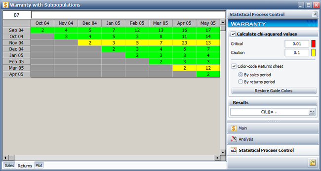
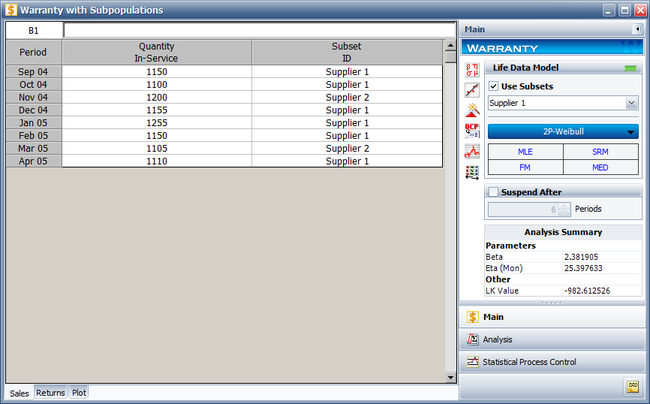
To analyze the warranty returns, select the check box in the Statistical Process Control page of the control panel and set the alpha values to 0.01 for the Critical Value and 0.1 for the Caution Value. Select to color code the results By sales period. The following figure shows the analysis settings and results of the analysis.

As you can see, the November 04 and March 05 sales periods are colored in yellow indicating that they are outlier sales periods, while the rest are green. One suspected reason for the variation may be the material used in production during these periods. Further analysis confirmed that for these periods, the material was acquired from a different supplier. This implies that the units are not homogenous, and that there are different sub-populations present in the field population.

Categorized each shipment (using the Subset ID column) based on their material supplier, as shown next. On the control panel, select the Use Subsets check box. Perform the analysis again using the two-parameter Weibull distribution and the MLE analysis method for both sub-populations.

The new models that describe the data are:

[math]\displaystyle{ \begin{matrix} Supplier 1 & Supplier 2 \\ \begin{matrix} \beta =2.381905 \\ \eta =25.397633 \\ \end{matrix} & \begin{matrix} \beta =2.320696 \\ \eta =21.282926 \\ \end{matrix} \\ \end{matrix}\,\! }[/math]

This analysis uncovered different sub-populations in the data set. Note that if the analysis were performed on the failure and suspension times in a regular standard folio using the mixed Weibull distribution, one would not be able to detect which units fall into which sub-population.

Warranty Analysis (Usage Format)

Warranty data analysis relies on the estimation of a failure distribution based on data including the number of returns and the number of surviving units in the field and the age associated with those units. The Usage Format allows the user to convert shipping and warranty return data into the standard reliability data for of failures and suspensions when the return information is based on usage rather than return dates or periods.

Suppose that you have been collecting sales (units in service) and returns data. For the returns data, you can determine the number of failures and their usage (by reading the odometer value, for example). Determining the number of surviving units (suspensions) and their ages is a straightforward step. By taking the difference between the analysis date and the date when a unit was put in service, you can determine the age of the surviving units.

What is unknown, however, is the exact usage accumulated by each surviving unit. The key part of the usage-based warranty analysis is the determination of the usage of the surviving units based on their age. Therefore, the analyst needs to have an idea about the usage of the product. This can be obtained, for example, from customer surveys or by designing the products to collect usage data. For example, in automotive applications, engineers often use 12,000 miles/year as an average usage. Based on this average, the usage of an item that has been in the field for 6 months and has not yet failed would be 6,000 miles. So to obtain the usage of a suspension based on an average usage, one could take the time of each suspension and multiply it by this average usage. As you see, in this situation the analysis becomes straightforward. With the usage values and the quantities of the returned units, a failure distribution can be constructed and subsequent warranty analysis becomes possible.

Alternatively, and more realistically, instead of using an average usage, an actual distribution that reflects the variation in usage and customer behavior can be used. This distribution describes the usage of a unit over a certain time period (e.g. 1 year, 1 month, etc). This probabilistic model can be used to estimate the usage for all surviving components in service and the percentage of users running the product at different usage rates. In the automotive example, for instance, such a distribution can be used to calculate the percentage of customers that drive 0-200 miles/month, 200-400 miles/month, etc. We can take these percentages and multiply them by the number of suspensions to find the number of items that have been accumulating usage values in these ranges.

To proceed with applying a usage distribution, the usage distribution is divided into increments based on a specified interval width denoted as [math]\displaystyle{ Z }[/math] . The usage distribution, [math]\displaystyle{ Q }[/math] , is divided into intervals of [math]\displaystyle{ 0+Z }[/math] , [math]\displaystyle{ Z+Z }[/math] , [math]\displaystyle{ 2Z+Z }[/math] , etc., or [math]\displaystyle{ {{x}_{i}}={{x}_{i-1}}+Z }[/math] , as shown in the next figure.

The interval width should be selected such that it creates segments that are large enough to contain adequate numbers of suspensions within the intervals.

The percentage of suspensions that belong to each usage interval is calculated as follows:

[math]\displaystyle{ F({{x}_{i}})=Q({{x}_{i}})-Q({{x}_{i}}-1) }[/math]

where:

[math]\displaystyle{ Q() }[/math] is the usage distribution Cumulative Density Function, [math]\displaystyle{ cdf }[/math] .

[math]\displaystyle{ x }[/math] represents the intervals used in apportioning the suspended population.

We also define a suspension group as a collection of suspensions that have the same age.

The above percentage of suspensions can be translated to numbers of suspensions within each interval, [math]\displaystyle{ {{x}_{i}} }[/math] . This is done by taking each group of suspensions and multiplying it by each [math]\displaystyle{ F({{x}_{i}}) }[/math] , or:

[math]\displaystyle{ \begin{align} & {{N}_{1,j}}= & F({{x}_{1}})\times N{{S}_{j}} \\ & {{N}_{2,j}}= & F({{x}_{2}})\times N{{S}_{j}} \\ & & ... \\ & {{N}_{n,j}}= & F({{x}_{n}})\times N{{S}_{j}} \end{align} }[/math]

where:

[math]\displaystyle{ {{N}_{n,j}} }[/math] is the number of suspensions that belong to each interval.

[math]\displaystyle{ N{{S}_{j}} }[/math] is the jth group of suspensions from the data set.

This is repeated for all the groups of suspensions.

The age of the suspensions is calculated by subtracting the Date In-Service ( [math]\displaystyle{ DIS }[/math] ), the date at which the unit started operation, from the calculation End Date ( [math]\displaystyle{ ED }[/math] ). This is the Time In-Service ( [math]\displaystyle{ TIS }[/math] ) value that describes the age of the surviving unit.

[math]\displaystyle{ TIS=ED-DIS }[/math]

Note: [math]\displaystyle{ TIS }[/math] is in the same time units as the period in which the usage distribution is defined.

For each [math]\displaystyle{ {{N}_{k,j}} }[/math] , the usage is calculated as:

[math]\displaystyle{ Uk,j=xi\times TISj }[/math]

After this step, the usage of each suspension group is estimated. The data can be combined with the failures and a failure distribution can be fitted.

Example 2: Warranty Analysis Usage Format Example

Suppose that an automotive manufacturer collects the warranty returns and sales data given in the following tables. Convert this information to life data and analyze it using the lognormal distribution.

Quality In-Service Data

Quantity In-Service	Date In-Service
9	Dec-09
13	Jan-10
15	Feb-10
20	Mar-10
15	Apr-10
25	May-10
19	Jun-10
16	Jul-10
20	Aug-10
19	Sep-10
25	Oct-10
30	Nov-10

Quality Return Data

Quantity Returned	Usage at Return Date	Date In-Service
1	9072	Dec-09
1	9743	Jan-10
1	6857	Feb-10
1	7651	Mar-10
1	5083	May-10
1	5990	May-10
1	7432	May-10
1	8739	May-10
1	3158	Jun-10
1	1136	Jul-10
1	4646	Aug-10
1	3965	Sep-10
1	3117	Oct-10
1	3250	Nov-10

Solution

Create a warranty analysis folio and select the usage format. Enter the data from the tables in the Sales, Returns and Future Sales sheets. The warranty data were collected until 12/1/2010; therefore, on the control panel, set the End of Observation Period to that date. Set the failure distribution to Lognormal, as shown next.

In this example, the manufacturer has been documenting the mileage accumulation per year for this type of product across the customer base in comparable regions for many years. The yearly usage has been determined to follow a lognormal distribution with [math]\displaystyle{ {{\mu }_{T\prime }}=9.38\,\! }[/math], [math]\displaystyle{ {{\sigma }_{T\prime }}=0.085\,\! }[/math]. The Interval Width is defined to be 1,000 miles. Enter the information about the usage distribution on the Suspensions page of the control panel, as shown next.

Click Calculate to analyze the data set. The parameters are estimated to be:

[math]\displaystyle{ \begin{align} & {{\mu }_{T\prime }}= & 10.528098 \\ & {{\sigma }_{T\prime }}= & 1.135150 \end{align}\,\! }[/math]

The reliability plot (with mileage being the random variable driving reliability), along with the 90% confidence bounds on reliability, is shown next.

In this example, the life data set contains 14 failures and 212 suspensions spread according to the defined usage distribution. You can display this data in a standard folio by choosing Warranty > Transfer Life Data > Transfer Life Data to New Folio. The failures and suspensions data set, as presented in the standard folio, is shown next (showing only the first 30 rows of data).

Warranty Prediction

Once a life data analysis has been performed on warranty data, this information can be used to predict how many warranty returns there will be in subsequent time periods. This methodology uses the concept of conditional reliability (see Chapter Basic Statistical Background) to calculate the probability of failure for the remaining units for each shipment time period. This conditional probability of failure is then multiplied by the number of units at risk from that particular shipment period that are still in the field (i.e. the suspensions) in order to predict the number of failures or warranty returns expected for this time period. The next example illustrates this.

Example 3:

The Warranty Analysis Folio in Weibull++ provides three different data entry formats for warranty data. It also allows the user to automatically perform a life data analysis on this type of data, allows the prediction of future failures through the use of conditional probability analysis and provides methods for detecting outliers.

Warranty Data Entry Types

Weibull++ allows for data entry utilizing four common formats for storing sales and returns information. Specifically:

1) Nevada Chart Format

2) Time-to-Failure Format

3) Dates of Failure Format

4) Usage Format

These formats are explained in the next sections.

Nevada Chart Format

Field information frequently appears in terms of units produced and/or shipped in a certain time period, with the resulting returns for that production lot in the subsequent time periods. This information can be arranged in a diagonal chart, as displayed in the following figure.

In Weibull++ this window is as shown next:

Time-to-Failure Format

This format is similar to the Standard Folio data entry format (all number of units, failure times and suspension times are entered by the user), as discussed previously. The difference is that when the data is used within the context of warranty analysis, the automatic ability to generate forecasts is available to the user. In Weibull++ this window is as shown next:

Dates of Failure Format

Another common way for reporting field information is to enter a date and quantity of sales or shipments, Quantity In-Service Data, and the date and quantity of returns, Quantity Returned Data, as illustrated in the following tables.

Quality In-Service Data

Quantity Returned Data

Note that in order to identify which lot the unit comes from, a failure is identified by a return date and the date of when it was put in service. The date that the unit went into service is then associated with the lot going into service during that time period. Lots can be used with the optional ID column which is covered in the sections that follow.

In Weibull++ this window is as shown next:

[math]\displaystyle{ }[/math]

Usage Format

Often the driving factor for reliability is usage rather than time. For example, in the automotive industry, the failure behavior in the majority of the products is mileage-dependent rather than time-dependent. This format allows specifying Quantity In-Service Data, and the usage at return date and Quantity Return Data, as illustrated in the following tables.

Quality In-Service Data

Note that, like in the dates of failure format, in order to identify which lot the unit comes from, a failure is identified by the return number and the date of when it was put in service. The date that the returned unit went into service associates the returned unit with the lot it belonged to when it started operation. However, the return data is in terms of usage and not date of return. Therefore the usage of the units needs to be specified as a constant usage per unit time or as a distribution. This allows determining the expected usage of the surviving units (See Example 2).

Warranty Analysis (Nevada Format)

The Nevada Format allows the user to convert shipping and warranty return data into the standard reliability data form of failures and suspensions so that it can easily be analyzed with traditional life data analysis methods. For each time period in which a number of products are shipped, there will be a certain number of returns or failures in subsequent time periods, while the rest of the population that was shipped will continue to operate in the following time periods. For example, if 500 units are shipped in May, and 10 of those units are warranty returns in June, that is equivalent to 10 failures at a time of one month. The other 450 units will go on to operate and possibly fail in months that follow. At the end of the analysis period, all of the units that were shipped and have not failed in the time since shipment are considered to be suspensions. This process is repeated for each shipment and the results tabulated for each particular failure and suspension time prior to reliability analysis. This process may sound confusing, but it is actually just a matter of careful bookkeeping, and is illustrated with the example that follows.

Example 1:

Warranty Analysis (Usage Format)

Warranty data analysis relies on the estimation of a failure distribution based on data including the number of returns and the number of surviving units in the field and the age associated with those units. The Usage Format allows the user to convert shipping and warranty return data into the standard reliability data for of failures and suspensions when the return information is based on usage rather than return dates or periods.

Suppose that you have been collecting sales (units in service) and returns data. For the returns data, you can determine the number of failures and their usage (by reading the odometer value, for example). Determining the number of surviving units (suspensions) and their ages is a straightforward step. By taking the difference between the analysis date and the date when a unit was put in service, you can determine the age of the surviving units.

What is unknown, however, is the exact usage accumulated by each surviving unit. The key part of the usage-based warranty analysis is the determination of the usage of the surviving units based on their age. Therefore, the analyst needs to have an idea about the usage of the product. This can be obtained, for example, from customer surveys or by designing the products to collect usage data. For example, in automotive applications, engineers often use 12,000 miles/year as an average usage. Based on this average, the usage of an item that has been in the field for 6 months and has not yet failed would be 6,000 miles. So to obtain the usage of a suspension based on an average usage, one could take the time of each suspension and multiply it by this average usage. As you see, in this situation the analysis becomes straightforward. With the usage values and the quantities of the returned units, a failure distribution can be constructed and subsequent warranty analysis becomes possible.

Alternatively, and more realistically, instead of using an average usage, an actual distribution that reflects the variation in usage and customer behavior can be used. This distribution describes the usage of a unit over a certain time period (e.g. 1 year, 1 month, etc). This probabilistic model can be used to estimate the usage for all surviving components in service and the percentage of users running the product at different usage rates. In the automotive example, for instance, such a distribution can be used to calculate the percentage of customers that drive 0-200 miles/month, 200-400 miles/month, etc. We can take these percentages and multiply them by the number of suspensions to find the number of items that have been accumulating usage values in these ranges.

To proceed with applying a usage distribution, the usage distribution is divided into increments based on a specified interval width denoted as [math]\displaystyle{ Z }[/math] . The usage distribution, [math]\displaystyle{ Q }[/math] , is divided into intervals of [math]\displaystyle{ 0+Z }[/math] , [math]\displaystyle{ Z+Z }[/math] , [math]\displaystyle{ 2Z+Z }[/math] , etc., or [math]\displaystyle{ {{x}_{i}}={{x}_{i-1}}+Z }[/math] , as shown in the next figure.

The interval width should be selected such that it creates segments that are large enough to contain adequate numbers of suspensions within the intervals.

The percentage of suspensions that belong to each usage interval is calculated as follows:

[math]\displaystyle{ F({{x}_{i}})=Q({{x}_{i}})-Q({{x}_{i}}-1) }[/math]

where:

[math]\displaystyle{ Q() }[/math] is the usage distribution Cumulative Density Function, [math]\displaystyle{ cdf }[/math] .

[math]\displaystyle{ x }[/math] represents the intervals used in apportioning the suspended population.

We also define a suspension group as a collection of suspensions that have the same age.

The above percentage of suspensions can be translated to numbers of suspensions within each interval, [math]\displaystyle{ {{x}_{i}} }[/math] . This is done by taking each group of suspensions and multiplying it by each [math]\displaystyle{ F({{x}_{i}}) }[/math] , or:

[math]\displaystyle{ \begin{align} & {{N}_{1,j}}= & F({{x}_{1}})\times N{{S}_{j}} \\ & {{N}_{2,j}}= & F({{x}_{2}})\times N{{S}_{j}} \\ & & ... \\ & {{N}_{n,j}}= & F({{x}_{n}})\times N{{S}_{j}} \end{align} }[/math]

where:

[math]\displaystyle{ {{N}_{n,j}} }[/math] is the number of suspensions that belong to each interval.

[math]\displaystyle{ N{{S}_{j}} }[/math] is the jth group of suspensions from the data set.

This is repeated for all the groups of suspensions.

The age of the suspensions is calculated by subtracting the Date In-Service ( [math]\displaystyle{ DIS }[/math] ), the date at which the unit started operation, from the calculation End Date ( [math]\displaystyle{ ED }[/math] ). This is the Time In-Service ( [math]\displaystyle{ TIS }[/math] ) value that describes the age of the surviving unit.

[math]\displaystyle{ TIS=ED-DIS }[/math]

Note: [math]\displaystyle{ TIS }[/math] is in the same time units as the period in which the usage distribution is defined.

For each [math]\displaystyle{ {{N}_{k,j}} }[/math] , the usage is calculated as:

[math]\displaystyle{ Uk,j=xi\times TISj }[/math]

After this step, the usage of each suspension group is estimated. The data can be combined with the failures and a failure distribution can be fitted.

Example 2: Warranty Analysis Usage Format Example

Suppose that an automotive manufacturer collects the warranty returns and sales data given in the following tables. Convert this information to life data and analyze it using the lognormal distribution.

Quality In-Service Data

Quantity In-Service	Date In-Service
9	Dec-09
13	Jan-10
15	Feb-10
20	Mar-10
15	Apr-10
25	May-10
19	Jun-10
16	Jul-10
20	Aug-10
19	Sep-10
25	Oct-10
30	Nov-10

Quality Return Data

Quantity Returned	Usage at Return Date	Date In-Service
1	9072	Dec-09
1	9743	Jan-10
1	6857	Feb-10
1	7651	Mar-10
1	5083	May-10
1	5990	May-10
1	7432	May-10
1	8739	May-10
1	3158	Jun-10
1	1136	Jul-10
1	4646	Aug-10
1	3965	Sep-10
1	3117	Oct-10
1	3250	Nov-10

Solution

Create a warranty analysis folio and select the usage format. Enter the data from the tables in the Sales, Returns and Future Sales sheets. The warranty data were collected until 12/1/2010; therefore, on the control panel, set the End of Observation Period to that date. Set the failure distribution to Lognormal, as shown next.

In this example, the manufacturer has been documenting the mileage accumulation per year for this type of product across the customer base in comparable regions for many years. The yearly usage has been determined to follow a lognormal distribution with [math]\displaystyle{ {{\mu }_{T\prime }}=9.38\,\! }[/math], [math]\displaystyle{ {{\sigma }_{T\prime }}=0.085\,\! }[/math]. The Interval Width is defined to be 1,000 miles. Enter the information about the usage distribution on the Suspensions page of the control panel, as shown next.

Click Calculate to analyze the data set. The parameters are estimated to be:

[math]\displaystyle{ \begin{align} & {{\mu }_{T\prime }}= & 10.528098 \\ & {{\sigma }_{T\prime }}= & 1.135150 \end{align}\,\! }[/math]

The reliability plot (with mileage being the random variable driving reliability), along with the 90% confidence bounds on reliability, is shown next.

In this example, the life data set contains 14 failures and 212 suspensions spread according to the defined usage distribution. You can display this data in a standard folio by choosing Warranty > Transfer Life Data > Transfer Life Data to New Folio. The failures and suspensions data set, as presented in the standard folio, is shown next (showing only the first 30 rows of data).

Warranty Prediction

Once a life data analysis has been performed on warranty data, this information can be used to predict how many warranty returns there will be in subsequent time periods. This methodology uses the concept of conditional reliability (see Chapter Basic Statistical Background) to calculate the probability of failure for the remaining units for each shipment time period. This conditional probability of failure is then multiplied by the number of units at risk from that particular shipment period that are still in the field (i.e. the suspensions) in order to predict the number of failures or warranty returns expected for this time period. The next example illustrates this.

Example 3:

Analysis of Non-Homogeneous Warranty Data

In the previous sections and examples it is important to note that the underlying assumption was that the population was homogeneous. In other words, all sold and returned units were exactly the same, i.e. the same population with no design changes and/or modifications. In many situations, as the product matures, design changes are made to enhance and/or improve the reliability of the product. Obviously, an improved product will exhibit different failure characteristics than its predecessor. To analyze such cases, where the population is non-homogeneous, one needs to extract each homogenous group, fit a life model to each group and then project the expected returns for each group based on the number of units at risk for each specific group.

Using IDs in Weibull++

Weibull++ uses the optional IDs column to differentiate between product versions or different designs (lots). Based on this entry, the data are then automatically separated and the parameters for each lot computed. Based on the computed parameters, failure projections can then be obtained. Note that it is important to realize that the same limitations as discussed previously, with regards to the number of failures that are needed, are also applicable here. In other words, distributions can be automatically fitted to lots that have return (failure) data, whereas if no returns have been experienced yet (either because the units are going to be introduced in the future or because no failures happened yet), the user will be asked to specify the parameters, since they can not be computed. Consequently, subsequent estimation/predictions related to these lots would be based on the user specified parameters. Following is an example that illustrates the use of IDs.

Example 4: Warranty Analysis Non-Homogeneous Data Example

A company keeps track of its production and returns. The company uses the dates of failure format to record the data. For the product in question, three versions (A, B and C) have been produced and put in service. The in-service data is as follows (using the Month/Day/Year date format):

[math]\displaystyle{ \begin{matrix} Quantity In-Service & Date of In-Service & ID \\ \text{400} & \text{1/1/2005} & \text{Model A} \\ \text{500} & \text{1/31/2005} & \text{Model A} \\ \text{500} & \text{5/1/2005} & \text{Model A} \\ \text{600} & \text{5/31/2005} & \text{Model A} \\ \text{550} & \text{6/30/2005} & \text{Model A} \\ \text{600} & \text{7/30/2005} & \text{Model A} \\ \text{800} & \text{9/28/2005} & \text{Model A} \\ \text{200} & \text{1/1/2005} & \text{Model B} \\ \text{350} & \text{3/2/2005} & \text{Model B} \\ \text{450} & \text{4/1/2005} & \text{Model B} \\ \text{300} & \text{6/30/2005} & \text{Model B} \\ \text{200} & \text{8/29/2005} & \text{Model B} \\ \text{350} & \text{10/28/2005} & \text{Model B} \\ \text{1100} & \text{2/1/2005} & \text{Model C} \\ \text{1200} & \text{3/27/2005} & \text{Model C} \\ \text{1200} & \text{4/25/2005} & \text{Model C} \\ \text{1300} & \text{6/1/2005} & \text{Model C} \\ \text{1400} & \text{8/26/2005} & \text{Model C} \\ \end{matrix}\,\! }[/math]

Furthermore, the following sales are forecast:

[math]\displaystyle{ \begin{matrix} Number & Date & ID \\ \text{400} & \text{6/27/2006} & \text{Model A} \\ \text{500} & \text{8/26/2006} & \text{Model A} \\ \text{550} & \text{10/26/2006} & \text{Model A} \\ \text{1200} & \text{7/25/2006} & \text{Model C} \\ \text{1300} & \text{9/27/2006} & \text{Model C} \\ \text{1250} & \text{11/26/2006} & \text{Model C} \\ \end{matrix}\,\! }[/math]

The return data are as follows. Note that in order to identify which lot each unit comes from, and to be able to compute its time-in-service, each return (failure) includes a return date, the date of when it was put in service and the model ID.

[math]\displaystyle{ \begin{matrix} Quantity Returned & Date of Return & Date In-Service & ID \\ \text{12} & \text{1/31/2005} & \text{1/1/2005} & \text{Model A} \\ \text{11} & \text{4/1/2005} & \text{1/31/2005} & \text{Model A} \\ \text{7} & \text{7/22/2005} & \text{5/1/2005} & \text{Model A} \\ \text{8} & \text{8/27/2005} & \text{5/31/2005} & \text{Model A} \\ \text{12} & \text{12/27/2005} & \text{5/31/2005} & \text{Model A} \\ \text{13} & \text{1/26/2006} & \text{6/30/2005} & \text{Model A} \\ \text{12} & \text{1/26/2006} & \text{7/30/2005} & \text{Model A} \\ \text{14} & \text{1/11/2006} & \text{9/28/2005} & \text{Model A} \\ \text{15} & \text{1/18/2006} & \text{9/28/2005} & \text{Model A} \\ \text{23} & \text{1/26/2005} & \text{1/1/2005} & \text{Model B} \\ \text{16} & \text{1/26/2005} & \text{1/1/2005} & \text{Model B} \\ \text{18} & \text{3/17/2005} & \text{1/1/2005} & \text{Model B} \\ \text{19} & \text{5/31/2005} & \text{3/2/2005} & \text{Model B} \\ \text{20} & \text{5/31/2005} & \text{3/2/2005} & \text{Model B} \\ \text{21} & \text{6/30/2005} & \text{3/2/2005} & \text{Model B} \\ \text{18} & \text{7/30/2005} & \text{4/1/2005} & \text{Model B} \\ \text{19} & \text{12/27/2005} & \text{6/30/2005} & \text{Model B} \\ \text{18} & \text{1/11/2006} & \text{8/29/2005} & \text{Model B} \\ \text{11} & \text{2/7/2006} & \text{10/28/2005} & \text{Model B} \\ \text{34} & \text{8/14/2005} & \text{3/27/2005} & \text{Model C} \\ \text{24} & \text{8/27/2005} & \text{4/25/2005} & \text{Model C} \\ \text{44} & \text{1/26/2006} & \text{6/1/2005} & \text{Model C} \\ \text{26} & \text{1/26/2006} & \text{8/26/2005} & \text{Model C} \\ \end{matrix}\,\! }[/math]

Assuming that the given information is current as of 5/1/2006, analyze the data using the lognormal distribution and MLE analysis method for all models (Model A, Model B, Model C), and provide a return forecast for the next ten months.

Solution

Create a warranty analysis folio and select the dates of failure format. Enter the data from the tables in the Sales, Returns and Future Sales sheets. On the control panel, select the Use Subsets check box, as shown next. This allows the software to separately analyze each subset of data. Use the drop-down list to switch between subset IDs and alter the analysis settings (use the lognormal distribution and MLE analysis method for all models).

In the End of Observation Period field, enter 5/1/2006, and then calculate the parameters. The results are:

[math]\displaystyle{ \begin{matrix} Model A & Model B & Model C \\ \begin{matrix} {{{\hat{\mu }}}^{\prime }}= & \text{11}\text{.28} \\ {{{\hat{\sigma }}}_{T}}= & \text{2}\text{.83} \\ \end{matrix} & \begin{matrix} {{{\hat{\mu }}}^{\prime }}= & \text{8}\text{.11} \\ {{{\hat{\sigma }}}_{T}}= & \text{2}\text{.30} \\ \end{matrix} & \begin{matrix} {{{\hat{\mu }}}^{\prime }}= & \text{9}\text{.79} \\ {{{\hat{\sigma }}}_{T}}= & \text{1}\text{.92} \\ \end{matrix} \\ \end{matrix}\,\! }[/math]

Note that in this example, the same distribution and analysis method were assumed for each of the product models. If desired, different distribution types, analysis methods, confidence bounds methods, etc., can be assumed for each IDs.

To obtain the expected failures for the next 10 months, click the Generate Forecast icon. In the Forecast Setup window, set the forecast to start on May 2, 2006 and set the number of forecast periods to 10. Set the increment (length of each period) to 1 Month, as shown next.

Click OK. A Forecast sheet will be created, with the predicted future returns. The following figure shows part of the Forecast sheet.

To view a summary of the analysis, click the Show Analysis Summary (...) button. The following figure shows the summary of the forecasted returns.

Click the Plot icon and choose the Expected Failures plot. The plot displays the predicted number of returns for each month, as shown next.

Monitoring Warranty Returns Using Statistical Process Control (SPC)

By monitoring and analyzing warranty return data, the user now has the ability to detect specific return periods and/or batches of sales or shipments that may deviate (differ) from the assumed model. This provides the analyst (and the organization) the advantage of early notification of possible deviations in manufacturing, use conditions and/or any other factor that may adversely affect the reliability of the fielded product.

Obviously, the motivation for performing such analysis is to allow for faster intervention to avoid increased costs due to increased warranty returns or more serious repercussions. Additionally, this analysis can also be used to uncover different sub-populations that may exist within this population.

Analysis Method

For each sales period [math]\displaystyle{ i }[/math] and return period [math]\displaystyle{ j }[/math] , the prediction error can be calculated as follows:

[math]\displaystyle{ {{e}_{i,j}}={{\hat{F}}_{i,j}}-{{F}_{i,j}} }[/math]

where [math]\displaystyle{ {{\hat{F}}_{i,j}} }[/math] is the estimated number of failures based on the estimated distribution parameters for the sales period [math]\displaystyle{ i }[/math] and the return period [math]\displaystyle{ j }[/math] , which is calculated using the equation for the conditional probability, and [math]\displaystyle{ {{F}_{i,j}} }[/math] is the actual number of failure for the sales period [math]\displaystyle{ i }[/math] and the return period [math]\displaystyle{ j }[/math] .

Since we are assuming that the model is accurate, [math]\displaystyle{ {{e}_{i,j}} }[/math] should follow a normal distribution with mean value of zero and a standard deviation [math]\displaystyle{ s }[/math] , where:

[math]\displaystyle{ {{\bar{e}}_{i,j}}=\frac{\underset{i}{\mathop{\sum }}\,\underset{j}{\mathop{\sum }}\,{{e}_{i,j}}}{n}=0 }[/math]

and [math]\displaystyle{ n }[/math] is the total number of return data (total number of residuals).

The estimated standard deviation of the prediction errors can then be calculated by:

[math]\displaystyle{ s=\sqrt{\frac{1}{n-1}\underset{i}{\mathop \sum }\,\underset{j}{\mathop \sum }\,e_{i,j}^{2}} }[/math]

and [math]\displaystyle{ {{e}_{i,j}} }[/math] can be normalized as follows:

[math]\displaystyle{ {{z}_{i,j}}=\frac{{{e}_{i,j}}}{s} }[/math]

where [math]\displaystyle{ {{z}_{i,j}} }[/math] is the standardized error. [math]\displaystyle{ {{z}_{i,j}} }[/math] follows a normal distribution with [math]\displaystyle{ \mu =0 }[/math] and [math]\displaystyle{ \sigma =1 }[/math] .

It is known that the square of a random variable with standard normal distribution follows the [math]\displaystyle{ {{\chi }^{2}} }[/math] (Chi Square) distribution with 1 degree of freedom and that the sum of the squares of [math]\displaystyle{ m }[/math] random variables with standard normal distribution follows the [math]\displaystyle{ {{\chi }^{2}} }[/math] distribution with [math]\displaystyle{ m }[/math] degrees of freedom [math]\displaystyle{ . }[/math] This then can be used to help detect the abnormal returns for a given sales period, return period or just a specific cell (combination of a return and a sales period).

• For a cell, abnormality is detected if [math]\displaystyle{ z_{i,j}^{2}=\chi _{1}^{2}\ge \chi _{1,\alpha }^{2}. }[/math]
• For an entire sales period [math]\displaystyle{ i }[/math] , abnormality is detected if [math]\displaystyle{ \underset{j}{\mathop{\sum }}\,z_{i,j}^{2}=\chi _{J}^{2}\ge \chi _{\alpha ,J}^{2}, }[/math] where [math]\displaystyle{ J }[/math] is the total number of return period for a sales period [math]\displaystyle{ i }[/math] .
• For an entire return period [math]\displaystyle{ j }[/math] , abnormality is detected if [math]\displaystyle{ \underset{i}{\mathop{\sum }}\,z_{i,j}^{2}=\chi _{I}^{2}\ge \chi _{\alpha ,I}^{2}, }[/math] where [math]\displaystyle{ I }[/math] is the total number of sales period for a return period [math]\displaystyle{ j }[/math] .

Here [math]\displaystyle{ \alpha }[/math] is the criticality value of the [math]\displaystyle{ {{\chi }^{2}} }[/math] distribution, which can be set at critical value or caution value. It describes the level of sensitivity to outliers (returns that deviate significantly from the predictions based on the fitted model). Increasing the value of [math]\displaystyle{ \alpha }[/math] increases the power of detection, but this could lead to more false alarms.

Example 5:

Example 6: Using Subset IDs with Statistical Process Control

A manufacturer wants to monitor and analyze the warranty returns for a particular product. They collected the following sales and return data.

[math]\displaystyle{ \begin{matrix} Period & Quantity In-Service \\ \text{Sep 04} & \text{1150} \\ \text{Oct 04} & \text{1100} \\ \text{Nov 04} & \text{1200} \\ \text{Dec 04} & \text{1155} \\ \text{Jan 05} & \text{1255} \\ \text{Feb 05} & \text{1150} \\ \text{Mar 05} & \text{1105} \\ \text{Apr 05} & \text{1110} \\ \end{matrix}\,\! }[/math]

[math]\displaystyle{ \begin{matrix} {} & Oct 04 & Nov 04 & Dec 04 & Jan 05 & Feb 05 & Mar 05 & Apr 05 & May 05 \\ Sep 05 & \text{2} & \text{4} & \text{5} & \text{7} & \text{12} & \text{13} & \text{16} & \text{17} \\ Oct 05 & \text{-} & \text{3} & \text{4} & \text{5} & \text{3} & \text{8} & \text{11} & \text{14} \\ Nov 05 & \text{-} & \text{-} & \text{2} & \text{3} & \text{5} & \text{7} & \text{23} & \text{13} \\ Dec 05 & \text{-} & \text{-} & \text{-} & \text{2} & \text{3} & \text{4} & \text{6} & \text{7} \\ Jan 06 & \text{-} & \text{-} & \text{-} & \text{-} & \text{2} & \text{3} & \text{3} & \text{4} \\ Feb 06 & \text{-} & \text{-} & \text{-} & \text{-} & \text{-} & \text{2} & \text{3} & \text{3} \\ Mar 06 & \text{-} & \text{-} & \text{-} & \text{-} & \text{-} & \text{-} & \text{2} & \text{12} \\ Apr 06 & \text{-} & \text{-} & \text{-} & \text{-} & \text{-} & \text{-} & \text{-} & \text{2} \\ \end{matrix}\,\! }[/math]

Solution

Analyze the data using the two-parameter Weibull distribution and the MLE analysis method. The parameters are estimated to be:

[math]\displaystyle{ \begin{align} & & \beta = & 2.318144 \\ & & \eta = & 25.071878 \end{align}\,\! }[/math]

To analyze the warranty returns, select the check box in the Statistical Process Control page of the control panel and set the alpha values to 0.01 for the Critical Value and 0.1 for the Caution Value. Select to color code the results By sales period. The following figure shows the analysis settings and results of the analysis.

As you can see, the November 04 and March 05 sales periods are colored in yellow indicating that they are outlier sales periods, while the rest are green. One suspected reason for the variation may be the material used in production during these periods. Further analysis confirmed that for these periods, the material was acquired from a different supplier. This implies that the units are not homogenous, and that there are different sub-populations present in the field population.

Categorized each shipment (using the Subset ID column) based on their material supplier, as shown next. On the control panel, select the Use Subsets check box. Perform the analysis again using the two-parameter Weibull distribution and the MLE analysis method for both sub-populations.

The new models that describe the data are:

[math]\displaystyle{ \begin{matrix} Supplier 1 & Supplier 2 \\ \begin{matrix} \beta =2.381905 \\ \eta =25.397633 \\ \end{matrix} & \begin{matrix} \beta =2.320696 \\ \eta =21.282926 \\ \end{matrix} \\ \end{matrix}\,\! }[/math]

This analysis uncovered different sub-populations in the data set. Note that if the analysis were performed on the failure and suspension times in a regular standard folio using the mixed Weibull distribution, one would not be able to detect which units fall into which sub-population.

Analysis of Non-Homogeneous Warranty Data

In the previous sections and examples it is important to note that the underlying assumption was that the population was homogeneous. In other words, all sold and returned units were exactly the same, i.e. the same population with no design changes and/or modifications. In many situations, as the product matures, design changes are made to enhance and/or improve the reliability of the product. Obviously, an improved product will exhibit different failure characteristics than its predecessor. To analyze such cases, where the population is non-homogeneous, one needs to extract each homogenous group, fit a life model to each group and then project the expected returns for each group based on the number of units at risk for each specific group.

Using IDs in Weibull++

Weibull++ uses the optional IDs column to differentiate between product versions or different designs (lots). Based on this entry, the data are then automatically separated and the parameters for each lot computed. Based on the computed parameters, failure projections can then be obtained. Note that it is important to realize that the same limitations as discussed previously, with regards to the number of failures that are needed, are also applicable here. In other words, distributions can be automatically fitted to lots that have return (failure) data, whereas if no returns have been experienced yet (either because the units are going to be introduced in the future or because no failures happened yet), the user will be asked to specify the parameters, since they can not be computed. Consequently, subsequent estimation/predictions related to these lots would be based on the user specified parameters. Following is an example that illustrates the use of IDs.

Example 4: Warranty Analysis Non-Homogeneous Data Example

A company keeps track of its production and returns. The company uses the dates of failure format to record the data. For the product in question, three versions (A, B and C) have been produced and put in service. The in-service data is as follows (using the Month/Day/Year date format):

[math]\displaystyle{ \begin{matrix} Quantity In-Service & Date of In-Service & ID \\ \text{400} & \text{1/1/2005} & \text{Model A} \\ \text{500} & \text{1/31/2005} & \text{Model A} \\ \text{500} & \text{5/1/2005} & \text{Model A} \\ \text{600} & \text{5/31/2005} & \text{Model A} \\ \text{550} & \text{6/30/2005} & \text{Model A} \\ \text{600} & \text{7/30/2005} & \text{Model A} \\ \text{800} & \text{9/28/2005} & \text{Model A} \\ \text{200} & \text{1/1/2005} & \text{Model B} \\ \text{350} & \text{3/2/2005} & \text{Model B} \\ \text{450} & \text{4/1/2005} & \text{Model B} \\ \text{300} & \text{6/30/2005} & \text{Model B} \\ \text{200} & \text{8/29/2005} & \text{Model B} \\ \text{350} & \text{10/28/2005} & \text{Model B} \\ \text{1100} & \text{2/1/2005} & \text{Model C} \\ \text{1200} & \text{3/27/2005} & \text{Model C} \\ \text{1200} & \text{4/25/2005} & \text{Model C} \\ \text{1300} & \text{6/1/2005} & \text{Model C} \\ \text{1400} & \text{8/26/2005} & \text{Model C} \\ \end{matrix}\,\! }[/math]

Furthermore, the following sales are forecast:

[math]\displaystyle{ \begin{matrix} Number & Date & ID \\ \text{400} & \text{6/27/2006} & \text{Model A} \\ \text{500} & \text{8/26/2006} & \text{Model A} \\ \text{550} & \text{10/26/2006} & \text{Model A} \\ \text{1200} & \text{7/25/2006} & \text{Model C} \\ \text{1300} & \text{9/27/2006} & \text{Model C} \\ \text{1250} & \text{11/26/2006} & \text{Model C} \\ \end{matrix}\,\! }[/math]

The return data are as follows. Note that in order to identify which lot each unit comes from, and to be able to compute its time-in-service, each return (failure) includes a return date, the date of when it was put in service and the model ID.

[math]\displaystyle{ \begin{matrix} Quantity Returned & Date of Return & Date In-Service & ID \\ \text{12} & \text{1/31/2005} & \text{1/1/2005} & \text{Model A} \\ \text{11} & \text{4/1/2005} & \text{1/31/2005} & \text{Model A} \\ \text{7} & \text{7/22/2005} & \text{5/1/2005} & \text{Model A} \\ \text{8} & \text{8/27/2005} & \text{5/31/2005} & \text{Model A} \\ \text{12} & \text{12/27/2005} & \text{5/31/2005} & \text{Model A} \\ \text{13} & \text{1/26/2006} & \text{6/30/2005} & \text{Model A} \\ \text{12} & \text{1/26/2006} & \text{7/30/2005} & \text{Model A} \\ \text{14} & \text{1/11/2006} & \text{9/28/2005} & \text{Model A} \\ \text{15} & \text{1/18/2006} & \text{9/28/2005} & \text{Model A} \\ \text{23} & \text{1/26/2005} & \text{1/1/2005} & \text{Model B} \\ \text{16} & \text{1/26/2005} & \text{1/1/2005} & \text{Model B} \\ \text{18} & \text{3/17/2005} & \text{1/1/2005} & \text{Model B} \\ \text{19} & \text{5/31/2005} & \text{3/2/2005} & \text{Model B} \\ \text{20} & \text{5/31/2005} & \text{3/2/2005} & \text{Model B} \\ \text{21} & \text{6/30/2005} & \text{3/2/2005} & \text{Model B} \\ \text{18} & \text{7/30/2005} & \text{4/1/2005} & \text{Model B} \\ \text{19} & \text{12/27/2005} & \text{6/30/2005} & \text{Model B} \\ \text{18} & \text{1/11/2006} & \text{8/29/2005} & \text{Model B} \\ \text{11} & \text{2/7/2006} & \text{10/28/2005} & \text{Model B} \\ \text{34} & \text{8/14/2005} & \text{3/27/2005} & \text{Model C} \\ \text{24} & \text{8/27/2005} & \text{4/25/2005} & \text{Model C} \\ \text{44} & \text{1/26/2006} & \text{6/1/2005} & \text{Model C} \\ \text{26} & \text{1/26/2006} & \text{8/26/2005} & \text{Model C} \\ \end{matrix}\,\! }[/math]

Assuming that the given information is current as of 5/1/2006, analyze the data using the lognormal distribution and MLE analysis method for all models (Model A, Model B, Model C), and provide a return forecast for the next ten months.

Solution

Create a warranty analysis folio and select the dates of failure format. Enter the data from the tables in the Sales, Returns and Future Sales sheets. On the control panel, select the Use Subsets check box, as shown next. This allows the software to separately analyze each subset of data. Use the drop-down list to switch between subset IDs and alter the analysis settings (use the lognormal distribution and MLE analysis method for all models).

In the End of Observation Period field, enter 5/1/2006, and then calculate the parameters. The results are:

[math]\displaystyle{ \begin{matrix} Model A & Model B & Model C \\ \begin{matrix} {{{\hat{\mu }}}^{\prime }}= & \text{11}\text{.28} \\ {{{\hat{\sigma }}}_{T}}= & \text{2}\text{.83} \\ \end{matrix} & \begin{matrix} {{{\hat{\mu }}}^{\prime }}= & \text{8}\text{.11} \\ {{{\hat{\sigma }}}_{T}}= & \text{2}\text{.30} \\ \end{matrix} & \begin{matrix} {{{\hat{\mu }}}^{\prime }}= & \text{9}\text{.79} \\ {{{\hat{\sigma }}}_{T}}= & \text{1}\text{.92} \\ \end{matrix} \\ \end{matrix}\,\! }[/math]

Note that in this example, the same distribution and analysis method were assumed for each of the product models. If desired, different distribution types, analysis methods, confidence bounds methods, etc., can be assumed for each IDs.

To obtain the expected failures for the next 10 months, click the Generate Forecast icon. In the Forecast Setup window, set the forecast to start on May 2, 2006 and set the number of forecast periods to 10. Set the increment (length of each period) to 1 Month, as shown next.

Click OK. A Forecast sheet will be created, with the predicted future returns. The following figure shows part of the Forecast sheet.

To view a summary of the analysis, click the Show Analysis Summary (...) button. The following figure shows the summary of the forecasted returns.

Click the Plot icon and choose the Expected Failures plot. The plot displays the predicted number of returns for each month, as shown next.

Monitoring Warranty Returns Using Statistical Process Control (SPC)

By monitoring and analyzing warranty return data, the user now has the ability to detect specific return periods and/or batches of sales or shipments that may deviate (differ) from the assumed model. This provides the analyst (and the organization) the advantage of early notification of possible deviations in manufacturing, use conditions and/or any other factor that may adversely affect the reliability of the fielded product.

Obviously, the motivation for performing such analysis is to allow for faster intervention to avoid increased costs due to increased warranty returns or more serious repercussions. Additionally, this analysis can also be used to uncover different sub-populations that may exist within this population.

Analysis Method

For each sales period [math]\displaystyle{ i }[/math] and return period [math]\displaystyle{ j }[/math] , the prediction error can be calculated as follows:

[math]\displaystyle{ {{e}_{i,j}}={{\hat{F}}_{i,j}}-{{F}_{i,j}} }[/math]

where [math]\displaystyle{ {{\hat{F}}_{i,j}} }[/math] is the estimated number of failures based on the estimated distribution parameters for the sales period [math]\displaystyle{ i }[/math] and the return period [math]\displaystyle{ j }[/math] , which is calculated using the equation for the conditional probability, and [math]\displaystyle{ {{F}_{i,j}} }[/math] is the actual number of failure for the sales period [math]\displaystyle{ i }[/math] and the return period [math]\displaystyle{ j }[/math] .

Since we are assuming that the model is accurate, [math]\displaystyle{ {{e}_{i,j}} }[/math] should follow a normal distribution with mean value of zero and a standard deviation [math]\displaystyle{ s }[/math] , where:

[math]\displaystyle{ {{\bar{e}}_{i,j}}=\frac{\underset{i}{\mathop{\sum }}\,\underset{j}{\mathop{\sum }}\,{{e}_{i,j}}}{n}=0 }[/math]

and [math]\displaystyle{ n }[/math] is the total number of return data (total number of residuals).

The estimated standard deviation of the prediction errors can then be calculated by:

[math]\displaystyle{ s=\sqrt{\frac{1}{n-1}\underset{i}{\mathop \sum }\,\underset{j}{\mathop \sum }\,e_{i,j}^{2}} }[/math]

and [math]\displaystyle{ {{e}_{i,j}} }[/math] can be normalized as follows:

[math]\displaystyle{ {{z}_{i,j}}=\frac{{{e}_{i,j}}}{s} }[/math]

where [math]\displaystyle{ {{z}_{i,j}} }[/math] is the standardized error. [math]\displaystyle{ {{z}_{i,j}} }[/math] follows a normal distribution with [math]\displaystyle{ \mu =0 }[/math] and [math]\displaystyle{ \sigma =1 }[/math] .

It is known that the square of a random variable with standard normal distribution follows the [math]\displaystyle{ {{\chi }^{2}} }[/math] (Chi Square) distribution with 1 degree of freedom and that the sum of the squares of [math]\displaystyle{ m }[/math] random variables with standard normal distribution follows the [math]\displaystyle{ {{\chi }^{2}} }[/math] distribution with [math]\displaystyle{ m }[/math] degrees of freedom [math]\displaystyle{ . }[/math] This then can be used to help detect the abnormal returns for a given sales period, return period or just a specific cell (combination of a return and a sales period).

• For a cell, abnormality is detected if [math]\displaystyle{ z_{i,j}^{2}=\chi _{1}^{2}\ge \chi _{1,\alpha }^{2}. }[/math]
• For an entire sales period [math]\displaystyle{ i }[/math] , abnormality is detected if [math]\displaystyle{ \underset{j}{\mathop{\sum }}\,z_{i,j}^{2}=\chi _{J}^{2}\ge \chi _{\alpha ,J}^{2}, }[/math] where [math]\displaystyle{ J }[/math] is the total number of return period for a sales period [math]\displaystyle{ i }[/math] .
• For an entire return period [math]\displaystyle{ j }[/math] , abnormality is detected if [math]\displaystyle{ \underset{i}{\mathop{\sum }}\,z_{i,j}^{2}=\chi _{I}^{2}\ge \chi _{\alpha ,I}^{2}, }[/math] where [math]\displaystyle{ I }[/math] is the total number of sales period for a return period [math]\displaystyle{ j }[/math] .

Here [math]\displaystyle{ \alpha }[/math] is the criticality value of the [math]\displaystyle{ {{\chi }^{2}} }[/math] distribution, which can be set at critical value or caution value. It describes the level of sensitivity to outliers (returns that deviate significantly from the predictions based on the fitted model). Increasing the value of [math]\displaystyle{ \alpha }[/math] increases the power of detection, but this could lead to more false alarms.

Example 5:

The Warranty Analysis Folio in Weibull++ provides three different data entry formats for warranty data. It also allows the user to automatically perform a life data analysis on this type of data, allows the prediction of future failures through the use of conditional probability analysis and provides methods for detecting outliers.

Warranty Data Entry Types

Weibull++ allows for data entry utilizing four common formats for storing sales and returns information. Specifically:

1) Nevada Chart Format

2) Time-to-Failure Format

3) Dates of Failure Format

4) Usage Format

These formats are explained in the next sections.

Nevada Chart Format

Field information frequently appears in terms of units produced and/or shipped in a certain time period, with the resulting returns for that production lot in the subsequent time periods. This information can be arranged in a diagonal chart, as displayed in the following figure.

In Weibull++ this window is as shown next:

Time-to-Failure Format

This format is similar to the Standard Folio data entry format (all number of units, failure times and suspension times are entered by the user), as discussed previously. The difference is that when the data is used within the context of warranty analysis, the automatic ability to generate forecasts is available to the user. In Weibull++ this window is as shown next:

Dates of Failure Format

Another common way for reporting field information is to enter a date and quantity of sales or shipments, Quantity In-Service Data, and the date and quantity of returns, Quantity Returned Data, as illustrated in the following tables.

Quality In-Service Data

Quantity Returned Data

Note that in order to identify which lot the unit comes from, a failure is identified by a return date and the date of when it was put in service. The date that the unit went into service is then associated with the lot going into service during that time period. Lots can be used with the optional ID column which is covered in the sections that follow.

In Weibull++ this window is as shown next:

[math]\displaystyle{ }[/math]

Usage Format

Often the driving factor for reliability is usage rather than time. For example, in the automotive industry, the failure behavior in the majority of the products is mileage-dependent rather than time-dependent. This format allows specifying Quantity In-Service Data, and the usage at return date and Quantity Return Data, as illustrated in the following tables.

Quality In-Service Data

Note that, like in the dates of failure format, in order to identify which lot the unit comes from, a failure is identified by the return number and the date of when it was put in service. The date that the returned unit went into service associates the returned unit with the lot it belonged to when it started operation. However, the return data is in terms of usage and not date of return. Therefore the usage of the units needs to be specified as a constant usage per unit time or as a distribution. This allows determining the expected usage of the surviving units (See Example 2).

Warranty Analysis (Nevada Format)

The Nevada Format allows the user to convert shipping and warranty return data into the standard reliability data form of failures and suspensions so that it can easily be analyzed with traditional life data analysis methods. For each time period in which a number of products are shipped, there will be a certain number of returns or failures in subsequent time periods, while the rest of the population that was shipped will continue to operate in the following time periods. For example, if 500 units are shipped in May, and 10 of those units are warranty returns in June, that is equivalent to 10 failures at a time of one month. The other 450 units will go on to operate and possibly fail in months that follow. At the end of the analysis period, all of the units that were shipped and have not failed in the time since shipment are considered to be suspensions. This process is repeated for each shipment and the results tabulated for each particular failure and suspension time prior to reliability analysis. This process may sound confusing, but it is actually just a matter of careful bookkeeping, and is illustrated with the example that follows.

Example 1:

Warranty Analysis (Usage Format)

Warranty data analysis relies on the estimation of a failure distribution based on data including the number of returns and the number of surviving units in the field and the age associated with those units. The Usage Format allows the user to convert shipping and warranty return data into the standard reliability data for of failures and suspensions when the return information is based on usage rather than return dates or periods.

Suppose that you have been collecting sales (units in service) and returns data. For the returns data, you can determine the number of failures and their usage (by reading the odometer value, for example). Determining the number of surviving units (suspensions) and their ages is a straightforward step. By taking the difference between the analysis date and the date when a unit was put in service, you can determine the age of the surviving units.

What is unknown, however, is the exact usage accumulated by each surviving unit. The key part of the usage-based warranty analysis is the determination of the usage of the surviving units based on their age. Therefore, the analyst needs to have an idea about the usage of the product. This can be obtained, for example, from customer surveys or by designing the products to collect usage data. For example, in automotive applications, engineers often use 12,000 miles/year as an average usage. Based on this average, the usage of an item that has been in the field for 6 months and has not yet failed would be 6,000 miles. So to obtain the usage of a suspension based on an average usage, one could take the time of each suspension and multiply it by this average usage. As you see, in this situation the analysis becomes straightforward. With the usage values and the quantities of the returned units, a failure distribution can be constructed and subsequent warranty analysis becomes possible.

Alternatively, and more realistically, instead of using an average usage, an actual distribution that reflects the variation in usage and customer behavior can be used. This distribution describes the usage of a unit over a certain time period (e.g. 1 year, 1 month, etc). This probabilistic model can be used to estimate the usage for all surviving components in service and the percentage of users running the product at different usage rates. In the automotive example, for instance, such a distribution can be used to calculate the percentage of customers that drive 0-200 miles/month, 200-400 miles/month, etc. We can take these percentages and multiply them by the number of suspensions to find the number of items that have been accumulating usage values in these ranges.

To proceed with applying a usage distribution, the usage distribution is divided into increments based on a specified interval width denoted as [math]\displaystyle{ Z }[/math] . The usage distribution, [math]\displaystyle{ Q }[/math] , is divided into intervals of [math]\displaystyle{ 0+Z }[/math] , [math]\displaystyle{ Z+Z }[/math] , [math]\displaystyle{ 2Z+Z }[/math] , etc., or [math]\displaystyle{ {{x}_{i}}={{x}_{i-1}}+Z }[/math] , as shown in the next figure.

The interval width should be selected such that it creates segments that are large enough to contain adequate numbers of suspensions within the intervals.

The percentage of suspensions that belong to each usage interval is calculated as follows:

[math]\displaystyle{ F({{x}_{i}})=Q({{x}_{i}})-Q({{x}_{i}}-1) }[/math]

where:

[math]\displaystyle{ Q() }[/math] is the usage distribution Cumulative Density Function, [math]\displaystyle{ cdf }[/math] .

[math]\displaystyle{ x }[/math] represents the intervals used in apportioning the suspended population.

We also define a suspension group as a collection of suspensions that have the same age.

The above percentage of suspensions can be translated to numbers of suspensions within each interval, [math]\displaystyle{ {{x}_{i}} }[/math] . This is done by taking each group of suspensions and multiplying it by each [math]\displaystyle{ F({{x}_{i}}) }[/math] , or:

[math]\displaystyle{ \begin{align} & {{N}_{1,j}}= & F({{x}_{1}})\times N{{S}_{j}} \\ & {{N}_{2,j}}= & F({{x}_{2}})\times N{{S}_{j}} \\ & & ... \\ & {{N}_{n,j}}= & F({{x}_{n}})\times N{{S}_{j}} \end{align} }[/math]

where:

[math]\displaystyle{ {{N}_{n,j}} }[/math] is the number of suspensions that belong to each interval.

[math]\displaystyle{ N{{S}_{j}} }[/math] is the jth group of suspensions from the data set.

This is repeated for all the groups of suspensions.

The age of the suspensions is calculated by subtracting the Date In-Service ( [math]\displaystyle{ DIS }[/math] ), the date at which the unit started operation, from the calculation End Date ( [math]\displaystyle{ ED }[/math] ). This is the Time In-Service ( [math]\displaystyle{ TIS }[/math] ) value that describes the age of the surviving unit.

[math]\displaystyle{ TIS=ED-DIS }[/math]

Note: [math]\displaystyle{ TIS }[/math] is in the same time units as the period in which the usage distribution is defined.

For each [math]\displaystyle{ {{N}_{k,j}} }[/math] , the usage is calculated as:

[math]\displaystyle{ Uk,j=xi\times TISj }[/math]

After this step, the usage of each suspension group is estimated. The data can be combined with the failures and a failure distribution can be fitted.

Example 2: Warranty Analysis Usage Format Example

Suppose that an automotive manufacturer collects the warranty returns and sales data given in the following tables. Convert this information to life data and analyze it using the lognormal distribution.

Quality In-Service Data

Quantity In-Service	Date In-Service
9	Dec-09
13	Jan-10
15	Feb-10
20	Mar-10
15	Apr-10
25	May-10
19	Jun-10
16	Jul-10
20	Aug-10
19	Sep-10
25	Oct-10
30	Nov-10

Quality Return Data

Quantity Returned	Usage at Return Date	Date In-Service
1	9072	Dec-09
1	9743	Jan-10
1	6857	Feb-10
1	7651	Mar-10
1	5083	May-10
1	5990	May-10
1	7432	May-10
1	8739	May-10
1	3158	Jun-10
1	1136	Jul-10
1	4646	Aug-10
1	3965	Sep-10
1	3117	Oct-10
1	3250	Nov-10

Solution

Create a warranty analysis folio and select the usage format. Enter the data from the tables in the Sales, Returns and Future Sales sheets. The warranty data were collected until 12/1/2010; therefore, on the control panel, set the End of Observation Period to that date. Set the failure distribution to Lognormal, as shown next.

In this example, the manufacturer has been documenting the mileage accumulation per year for this type of product across the customer base in comparable regions for many years. The yearly usage has been determined to follow a lognormal distribution with [math]\displaystyle{ {{\mu }_{T\prime }}=9.38\,\! }[/math], [math]\displaystyle{ {{\sigma }_{T\prime }}=0.085\,\! }[/math]. The Interval Width is defined to be 1,000 miles. Enter the information about the usage distribution on the Suspensions page of the control panel, as shown next.

Click Calculate to analyze the data set. The parameters are estimated to be:

[math]\displaystyle{ \begin{align} & {{\mu }_{T\prime }}= & 10.528098 \\ & {{\sigma }_{T\prime }}= & 1.135150 \end{align}\,\! }[/math]

The reliability plot (with mileage being the random variable driving reliability), along with the 90% confidence bounds on reliability, is shown next.

In this example, the life data set contains 14 failures and 212 suspensions spread according to the defined usage distribution. You can display this data in a standard folio by choosing Warranty > Transfer Life Data > Transfer Life Data to New Folio. The failures and suspensions data set, as presented in the standard folio, is shown next (showing only the first 30 rows of data).

Warranty Prediction

Once a life data analysis has been performed on warranty data, this information can be used to predict how many warranty returns there will be in subsequent time periods. This methodology uses the concept of conditional reliability (see Chapter Basic Statistical Background) to calculate the probability of failure for the remaining units for each shipment time period. This conditional probability of failure is then multiplied by the number of units at risk from that particular shipment period that are still in the field (i.e. the suspensions) in order to predict the number of failures or warranty returns expected for this time period. The next example illustrates this.

Example 3:

Analysis of Non-Homogeneous Warranty Data

In the previous sections and examples it is important to note that the underlying assumption was that the population was homogeneous. In other words, all sold and returned units were exactly the same, i.e. the same population with no design changes and/or modifications. In many situations, as the product matures, design changes are made to enhance and/or improve the reliability of the product. Obviously, an improved product will exhibit different failure characteristics than its predecessor. To analyze such cases, where the population is non-homogeneous, one needs to extract each homogenous group, fit a life model to each group and then project the expected returns for each group based on the number of units at risk for each specific group.

Using IDs in Weibull++

Weibull++ uses the optional IDs column to differentiate between product versions or different designs (lots). Based on this entry, the data are then automatically separated and the parameters for each lot computed. Based on the computed parameters, failure projections can then be obtained. Note that it is important to realize that the same limitations as discussed previously, with regards to the number of failures that are needed, are also applicable here. In other words, distributions can be automatically fitted to lots that have return (failure) data, whereas if no returns have been experienced yet (either because the units are going to be introduced in the future or because no failures happened yet), the user will be asked to specify the parameters, since they can not be computed. Consequently, subsequent estimation/predictions related to these lots would be based on the user specified parameters. Following is an example that illustrates the use of IDs.

Example 4: Warranty Analysis Non-Homogeneous Data Example

A company keeps track of its production and returns. The company uses the dates of failure format to record the data. For the product in question, three versions (A, B and C) have been produced and put in service. The in-service data is as follows (using the Month/Day/Year date format):

[math]\displaystyle{ \begin{matrix} Quantity In-Service & Date of In-Service & ID \\ \text{400} & \text{1/1/2005} & \text{Model A} \\ \text{500} & \text{1/31/2005} & \text{Model A} \\ \text{500} & \text{5/1/2005} & \text{Model A} \\ \text{600} & \text{5/31/2005} & \text{Model A} \\ \text{550} & \text{6/30/2005} & \text{Model A} \\ \text{600} & \text{7/30/2005} & \text{Model A} \\ \text{800} & \text{9/28/2005} & \text{Model A} \\ \text{200} & \text{1/1/2005} & \text{Model B} \\ \text{350} & \text{3/2/2005} & \text{Model B} \\ \text{450} & \text{4/1/2005} & \text{Model B} \\ \text{300} & \text{6/30/2005} & \text{Model B} \\ \text{200} & \text{8/29/2005} & \text{Model B} \\ \text{350} & \text{10/28/2005} & \text{Model B} \\ \text{1100} & \text{2/1/2005} & \text{Model C} \\ \text{1200} & \text{3/27/2005} & \text{Model C} \\ \text{1200} & \text{4/25/2005} & \text{Model C} \\ \text{1300} & \text{6/1/2005} & \text{Model C} \\ \text{1400} & \text{8/26/2005} & \text{Model C} \\ \end{matrix}\,\! }[/math]

Furthermore, the following sales are forecast:

[math]\displaystyle{ \begin{matrix} Number & Date & ID \\ \text{400} & \text{6/27/2006} & \text{Model A} \\ \text{500} & \text{8/26/2006} & \text{Model A} \\ \text{550} & \text{10/26/2006} & \text{Model A} \\ \text{1200} & \text{7/25/2006} & \text{Model C} \\ \text{1300} & \text{9/27/2006} & \text{Model C} \\ \text{1250} & \text{11/26/2006} & \text{Model C} \\ \end{matrix}\,\! }[/math]

The return data are as follows. Note that in order to identify which lot each unit comes from, and to be able to compute its time-in-service, each return (failure) includes a return date, the date of when it was put in service and the model ID.

[math]\displaystyle{ \begin{matrix} Quantity Returned & Date of Return & Date In-Service & ID \\ \text{12} & \text{1/31/2005} & \text{1/1/2005} & \text{Model A} \\ \text{11} & \text{4/1/2005} & \text{1/31/2005} & \text{Model A} \\ \text{7} & \text{7/22/2005} & \text{5/1/2005} & \text{Model A} \\ \text{8} & \text{8/27/2005} & \text{5/31/2005} & \text{Model A} \\ \text{12} & \text{12/27/2005} & \text{5/31/2005} & \text{Model A} \\ \text{13} & \text{1/26/2006} & \text{6/30/2005} & \text{Model A} \\ \text{12} & \text{1/26/2006} & \text{7/30/2005} & \text{Model A} \\ \text{14} & \text{1/11/2006} & \text{9/28/2005} & \text{Model A} \\ \text{15} & \text{1/18/2006} & \text{9/28/2005} & \text{Model A} \\ \text{23} & \text{1/26/2005} & \text{1/1/2005} & \text{Model B} \\ \text{16} & \text{1/26/2005} & \text{1/1/2005} & \text{Model B} \\ \text{18} & \text{3/17/2005} & \text{1/1/2005} & \text{Model B} \\ \text{19} & \text{5/31/2005} & \text{3/2/2005} & \text{Model B} \\ \text{20} & \text{5/31/2005} & \text{3/2/2005} & \text{Model B} \\ \text{21} & \text{6/30/2005} & \text{3/2/2005} & \text{Model B} \\ \text{18} & \text{7/30/2005} & \text{4/1/2005} & \text{Model B} \\ \text{19} & \text{12/27/2005} & \text{6/30/2005} & \text{Model B} \\ \text{18} & \text{1/11/2006} & \text{8/29/2005} & \text{Model B} \\ \text{11} & \text{2/7/2006} & \text{10/28/2005} & \text{Model B} \\ \text{34} & \text{8/14/2005} & \text{3/27/2005} & \text{Model C} \\ \text{24} & \text{8/27/2005} & \text{4/25/2005} & \text{Model C} \\ \text{44} & \text{1/26/2006} & \text{6/1/2005} & \text{Model C} \\ \text{26} & \text{1/26/2006} & \text{8/26/2005} & \text{Model C} \\ \end{matrix}\,\! }[/math]

Assuming that the given information is current as of 5/1/2006, analyze the data using the lognormal distribution and MLE analysis method for all models (Model A, Model B, Model C), and provide a return forecast for the next ten months.

Solution

Create a warranty analysis folio and select the dates of failure format. Enter the data from the tables in the Sales, Returns and Future Sales sheets. On the control panel, select the Use Subsets check box, as shown next. This allows the software to separately analyze each subset of data. Use the drop-down list to switch between subset IDs and alter the analysis settings (use the lognormal distribution and MLE analysis method for all models).

In the End of Observation Period field, enter 5/1/2006, and then calculate the parameters. The results are:

[math]\displaystyle{ \begin{matrix} Model A & Model B & Model C \\ \begin{matrix} {{{\hat{\mu }}}^{\prime }}= & \text{11}\text{.28} \\ {{{\hat{\sigma }}}_{T}}= & \text{2}\text{.83} \\ \end{matrix} & \begin{matrix} {{{\hat{\mu }}}^{\prime }}= & \text{8}\text{.11} \\ {{{\hat{\sigma }}}_{T}}= & \text{2}\text{.30} \\ \end{matrix} & \begin{matrix} {{{\hat{\mu }}}^{\prime }}= & \text{9}\text{.79} \\ {{{\hat{\sigma }}}_{T}}= & \text{1}\text{.92} \\ \end{matrix} \\ \end{matrix}\,\! }[/math]

Note that in this example, the same distribution and analysis method were assumed for each of the product models. If desired, different distribution types, analysis methods, confidence bounds methods, etc., can be assumed for each IDs.

To obtain the expected failures for the next 10 months, click the Generate Forecast icon. In the Forecast Setup window, set the forecast to start on May 2, 2006 and set the number of forecast periods to 10. Set the increment (length of each period) to 1 Month, as shown next.

Click OK. A Forecast sheet will be created, with the predicted future returns. The following figure shows part of the Forecast sheet.

To view a summary of the analysis, click the Show Analysis Summary (...) button. The following figure shows the summary of the forecasted returns.

Click the Plot icon and choose the Expected Failures plot. The plot displays the predicted number of returns for each month, as shown next.

Monitoring Warranty Returns Using Statistical Process Control (SPC)

By monitoring and analyzing warranty return data, the user now has the ability to detect specific return periods and/or batches of sales or shipments that may deviate (differ) from the assumed model. This provides the analyst (and the organization) the advantage of early notification of possible deviations in manufacturing, use conditions and/or any other factor that may adversely affect the reliability of the fielded product.

Obviously, the motivation for performing such analysis is to allow for faster intervention to avoid increased costs due to increased warranty returns or more serious repercussions. Additionally, this analysis can also be used to uncover different sub-populations that may exist within this population.

Analysis Method

For each sales period [math]\displaystyle{ i }[/math] and return period [math]\displaystyle{ j }[/math] , the prediction error can be calculated as follows:

[math]\displaystyle{ {{e}_{i,j}}={{\hat{F}}_{i,j}}-{{F}_{i,j}} }[/math]

where [math]\displaystyle{ {{\hat{F}}_{i,j}} }[/math] is the estimated number of failures based on the estimated distribution parameters for the sales period [math]\displaystyle{ i }[/math] and the return period [math]\displaystyle{ j }[/math] , which is calculated using the equation for the conditional probability, and [math]\displaystyle{ {{F}_{i,j}} }[/math] is the actual number of failure for the sales period [math]\displaystyle{ i }[/math] and the return period [math]\displaystyle{ j }[/math] .

Since we are assuming that the model is accurate, [math]\displaystyle{ {{e}_{i,j}} }[/math] should follow a normal distribution with mean value of zero and a standard deviation [math]\displaystyle{ s }[/math] , where:

[math]\displaystyle{ {{\bar{e}}_{i,j}}=\frac{\underset{i}{\mathop{\sum }}\,\underset{j}{\mathop{\sum }}\,{{e}_{i,j}}}{n}=0 }[/math]

and [math]\displaystyle{ n }[/math] is the total number of return data (total number of residuals).

The estimated standard deviation of the prediction errors can then be calculated by:

[math]\displaystyle{ s=\sqrt{\frac{1}{n-1}\underset{i}{\mathop \sum }\,\underset{j}{\mathop \sum }\,e_{i,j}^{2}} }[/math]

and [math]\displaystyle{ {{e}_{i,j}} }[/math] can be normalized as follows:

[math]\displaystyle{ {{z}_{i,j}}=\frac{{{e}_{i,j}}}{s} }[/math]

where [math]\displaystyle{ {{z}_{i,j}} }[/math] is the standardized error. [math]\displaystyle{ {{z}_{i,j}} }[/math] follows a normal distribution with [math]\displaystyle{ \mu =0 }[/math] and [math]\displaystyle{ \sigma =1 }[/math] .

It is known that the square of a random variable with standard normal distribution follows the [math]\displaystyle{ {{\chi }^{2}} }[/math] (Chi Square) distribution with 1 degree of freedom and that the sum of the squares of [math]\displaystyle{ m }[/math] random variables with standard normal distribution follows the [math]\displaystyle{ {{\chi }^{2}} }[/math] distribution with [math]\displaystyle{ m }[/math] degrees of freedom [math]\displaystyle{ . }[/math] This then can be used to help detect the abnormal returns for a given sales period, return period or just a specific cell (combination of a return and a sales period).

• For a cell, abnormality is detected if [math]\displaystyle{ z_{i,j}^{2}=\chi _{1}^{2}\ge \chi _{1,\alpha }^{2}. }[/math]
• For an entire sales period [math]\displaystyle{ i }[/math] , abnormality is detected if [math]\displaystyle{ \underset{j}{\mathop{\sum }}\,z_{i,j}^{2}=\chi _{J}^{2}\ge \chi _{\alpha ,J}^{2}, }[/math] where [math]\displaystyle{ J }[/math] is the total number of return period for a sales period [math]\displaystyle{ i }[/math] .
• For an entire return period [math]\displaystyle{ j }[/math] , abnormality is detected if [math]\displaystyle{ \underset{i}{\mathop{\sum }}\,z_{i,j}^{2}=\chi _{I}^{2}\ge \chi _{\alpha ,I}^{2}, }[/math] where [math]\displaystyle{ I }[/math] is the total number of sales period for a return period [math]\displaystyle{ j }[/math] .

Here [math]\displaystyle{ \alpha }[/math] is the criticality value of the [math]\displaystyle{ {{\chi }^{2}} }[/math] distribution, which can be set at critical value or caution value. It describes the level of sensitivity to outliers (returns that deviate significantly from the predictions based on the fitted model). Increasing the value of [math]\displaystyle{ \alpha }[/math] increases the power of detection, but this could lead to more false alarms.

Example 5:

Example 6: Using Subset IDs with Statistical Process Control

A manufacturer wants to monitor and analyze the warranty returns for a particular product. They collected the following sales and return data.

[math]\displaystyle{ \begin{matrix} Period & Quantity In-Service \\ \text{Sep 04} & \text{1150} \\ \text{Oct 04} & \text{1100} \\ \text{Nov 04} & \text{1200} \\ \text{Dec 04} & \text{1155} \\ \text{Jan 05} & \text{1255} \\ \text{Feb 05} & \text{1150} \\ \text{Mar 05} & \text{1105} \\ \text{Apr 05} & \text{1110} \\ \end{matrix}\,\! }[/math]

[math]\displaystyle{ \begin{matrix} {} & Oct 04 & Nov 04 & Dec 04 & Jan 05 & Feb 05 & Mar 05 & Apr 05 & May 05 \\ Sep 05 & \text{2} & \text{4} & \text{5} & \text{7} & \text{12} & \text{13} & \text{16} & \text{17} \\ Oct 05 & \text{-} & \text{3} & \text{4} & \text{5} & \text{3} & \text{8} & \text{11} & \text{14} \\ Nov 05 & \text{-} & \text{-} & \text{2} & \text{3} & \text{5} & \text{7} & \text{23} & \text{13} \\ Dec 05 & \text{-} & \text{-} & \text{-} & \text{2} & \text{3} & \text{4} & \text{6} & \text{7} \\ Jan 06 & \text{-} & \text{-} & \text{-} & \text{-} & \text{2} & \text{3} & \text{3} & \text{4} \\ Feb 06 & \text{-} & \text{-} & \text{-} & \text{-} & \text{-} & \text{2} & \text{3} & \text{3} \\ Mar 06 & \text{-} & \text{-} & \text{-} & \text{-} & \text{-} & \text{-} & \text{2} & \text{12} \\ Apr 06 & \text{-} & \text{-} & \text{-} & \text{-} & \text{-} & \text{-} & \text{-} & \text{2} \\ \end{matrix}\,\! }[/math]

Solution

Analyze the data using the two-parameter Weibull distribution and the MLE analysis method. The parameters are estimated to be:

[math]\displaystyle{ \begin{align} & & \beta = & 2.318144 \\ & & \eta = & 25.071878 \end{align}\,\! }[/math]

To analyze the warranty returns, select the check box in the Statistical Process Control page of the control panel and set the alpha values to 0.01 for the Critical Value and 0.1 for the Caution Value. Select to color code the results By sales period. The following figure shows the analysis settings and results of the analysis.

As you can see, the November 04 and March 05 sales periods are colored in yellow indicating that they are outlier sales periods, while the rest are green. One suspected reason for the variation may be the material used in production during these periods. Further analysis confirmed that for these periods, the material was acquired from a different supplier. This implies that the units are not homogenous, and that there are different sub-populations present in the field population.

Categorized each shipment (using the Subset ID column) based on their material supplier, as shown next. On the control panel, select the Use Subsets check box. Perform the analysis again using the two-parameter Weibull distribution and the MLE analysis method for both sub-populations.

The new models that describe the data are:

[math]\displaystyle{ \begin{matrix} Supplier 1 & Supplier 2 \\ \begin{matrix} \beta =2.381905 \\ \eta =25.397633 \\ \end{matrix} & \begin{matrix} \beta =2.320696 \\ \eta =21.282926 \\ \end{matrix} \\ \end{matrix}\,\! }[/math]

This analysis uncovered different sub-populations in the data set. Note that if the analysis were performed on the failure and suspension times in a regular standard folio using the mixed Weibull distribution, one would not be able to detect which units fall into which sub-population.

Example 6: Using Subset IDs with Statistical Process Control

A manufacturer wants to monitor and analyze the warranty returns for a particular product. They collected the following sales and return data.

[math]\displaystyle{ \begin{matrix} Period & Quantity In-Service \\ \text{Sep 04} & \text{1150} \\ \text{Oct 04} & \text{1100} \\ \text{Nov 04} & \text{1200} \\ \text{Dec 04} & \text{1155} \\ \text{Jan 05} & \text{1255} \\ \text{Feb 05} & \text{1150} \\ \text{Mar 05} & \text{1105} \\ \text{Apr 05} & \text{1110} \\ \end{matrix}\,\! }[/math]

[math]\displaystyle{ \begin{matrix} {} & Oct 04 & Nov 04 & Dec 04 & Jan 05 & Feb 05 & Mar 05 & Apr 05 & May 05 \\ Sep 05 & \text{2} & \text{4} & \text{5} & \text{7} & \text{12} & \text{13} & \text{16} & \text{17} \\ Oct 05 & \text{-} & \text{3} & \text{4} & \text{5} & \text{3} & \text{8} & \text{11} & \text{14} \\ Nov 05 & \text{-} & \text{-} & \text{2} & \text{3} & \text{5} & \text{7} & \text{23} & \text{13} \\ Dec 05 & \text{-} & \text{-} & \text{-} & \text{2} & \text{3} & \text{4} & \text{6} & \text{7} \\ Jan 06 & \text{-} & \text{-} & \text{-} & \text{-} & \text{2} & \text{3} & \text{3} & \text{4} \\ Feb 06 & \text{-} & \text{-} & \text{-} & \text{-} & \text{-} & \text{2} & \text{3} & \text{3} \\ Mar 06 & \text{-} & \text{-} & \text{-} & \text{-} & \text{-} & \text{-} & \text{2} & \text{12} \\ Apr 06 & \text{-} & \text{-} & \text{-} & \text{-} & \text{-} & \text{-} & \text{-} & \text{2} \\ \end{matrix}\,\! }[/math]

Solution

Analyze the data using the two-parameter Weibull distribution and the MLE analysis method. The parameters are estimated to be:

[math]\displaystyle{ \begin{align} & & \beta = & 2.318144 \\ & & \eta = & 25.071878 \end{align}\,\! }[/math]

To analyze the warranty returns, select the check box in the Statistical Process Control page of the control panel and set the alpha values to 0.01 for the Critical Value and 0.1 for the Caution Value. Select to color code the results By sales period. The following figure shows the analysis settings and results of the analysis.

As you can see, the November 04 and March 05 sales periods are colored in yellow indicating that they are outlier sales periods, while the rest are green. One suspected reason for the variation may be the material used in production during these periods. Further analysis confirmed that for these periods, the material was acquired from a different supplier. This implies that the units are not homogenous, and that there are different sub-populations present in the field population.

Categorized each shipment (using the Subset ID column) based on their material supplier, as shown next. On the control panel, select the Use Subsets check box. Perform the analysis again using the two-parameter Weibull distribution and the MLE analysis method for both sub-populations.

The new models that describe the data are:

[math]\displaystyle{ \begin{matrix} Supplier 1 & Supplier 2 \\ \begin{matrix} \beta =2.381905 \\ \eta =25.397633 \\ \end{matrix} & \begin{matrix} \beta =2.320696 \\ \eta =21.282926 \\ \end{matrix} \\ \end{matrix}\,\! }[/math]

This analysis uncovered different sub-populations in the data set. Note that if the analysis were performed on the failure and suspension times in a regular standard folio using the mixed Weibull distribution, one would not be able to detect which units fall into which sub-population.