Template:Probability Plotting

Probability Plotting

The least mathematically intensive method for parameter estimation is the method of probability plotting. As the term implies, probability plotting involves a physical plot of the data on specially constructed probability plotting paper. This method is easily implemented by hand, given that one can obtain the appropriate probability plotting paper.

Illustrating the Method for the 2-Parameter Weibull Distribution

The method of probability plotting takes the cdf of the distribution and attempts to linearize it by employing a specially constructed paper. This is best illustrated using the 2-parameter Weibull distribution.

In the case of the two-parameter Weibull distribution, the cdf (also the unreliability Q(t)) is given by:

[math]\displaystyle{ F(t)=Q(t)=1-{e^{-\left(\tfrac{t}{\eta}\right)^{\beta}}} }[/math]

Linearizing the Weibull Unreliability Function
This function can then be linearized (i.e., put in the common form of y = m'x + bformat) as follows:

[math]\displaystyle{ \begin{align} Q(t)= & 1-{e^{-\left(\tfrac{t}{\eta}\right)^{\beta}}} \\ \ln (1-Q(t))= & \ln \left[ {e^{-\left(\tfrac{t}{\eta}\right)^{\beta}}} \right] \\ \ln (1-Q(t))=& -\left(\tfrac{t}{\eta}\right)^{\beta} \\ \ln ( -\ln (1-Q(t)))= & \beta \left(\ln \left( \frac{t}{\eta }\right)\right) \\ \ln \left( \ln \left( \frac{1}{1-Q(t)}\right) \right) = & \beta\ln{ t} -\beta(\eta ) \\ \end{align} }[/math]

Then by setting

[math]\displaystyle{ y=\ln \left( \ln \left( \frac{1}{1-Q(t)} \right) \right) }[/math]

and

[math]\displaystyle{ x=\ln \left( t \right) }[/math]

the equation can then be rewritten as

[math]\displaystyle{ y=\beta x-\beta \ln \left( \eta \right) }[/math]

which is now a linear equation with a slope of

Slope = m = β

and an intercept of

Intercept[math]\displaystyle{ =b=-\beta \cdot ln(\eta) }[/math].

Constructing the Paper

The next task is to construct the Weibull probability plotting paper with the appropriate y - and x-axes. The x-axis trasnformation is simply logarithmic. The y-axis, is a bit more complex requiring a double log reciprocal transformation, or 

[math]\displaystyle{ y=\ln \left(\ln \left( \frac{1}{1-Q(t)} ) \right) \right) }[/math]

where Q(t) is the unreliability.

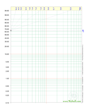
Such papers have been created by different vendors and are called probability plotting papers. Weibull.com has different plotting papers available for download.

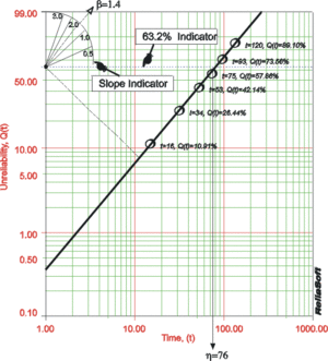
To illustrate, consider the following probability plot on a slightly different type of Weibull probability paper.

This paper is constructed based on the mentioned y - and x-transformations, where the y-axis represents unreliability and the x-axis represents time. Both of these values must be known for each time-to-failure point we want to plot.

Then, given the y and x value for each point, the points can easily be put on the plot. Once the points have been placed on the plot, the best possible straight line is drawn through these points. Once the line has been drawn, the slope of the line can be obtained (some probability papers include a slope indicator to simplify this calculation). This is the parameter β, which is the value of the slope. To determine the scale parameter, η (also called the characteristic life), one reads the time from the x-axis corresponding to Q(t)=63.2%.

Note that from before at

[math]\displaystyle{ \begin{align} Q(t=\eta)= & 1-{{e}^{-{{\left( \tfrac{t}{\eta } \right)}^{\beta }}}} \\ = & 1-{{e}^{-1}} \\ = & 0.632 \\ = & 63.2% \end{align} }[/math]

Thus, if we enter the y axis at Q(t)=63.2%, the corresponding value of t will be equal to η. Thus, using this simple methodology, the parameters of the Weibull distribution can be estimated.

Determining the x and y Position of the Plot Points

The points on the plot represent our data or, more specifically, our times-to-failure data. If, for example, we tested four units that failed at 10, 20, 30 and 40 hours, we would use these times as our x values or time values.

Determining what the appropriate y plotting positions, or the unreliability values, is a little more complex. To determine the y plotting positions, we must first determine a value indicating the corresponding unreliability for that failure. In other words, we need to obtain the cumulative percent failed for each time-to-failure. In this example, and by 10 hours, the cumulative percent failed is 25%, by 20 hours 50%, and so forth. This is a simple method illustrating the idea. The problem with this simple method is the fact that the 100% point is not defined on most probability plots, thus an alternative and more robust approach must be used. The most widely used method of determining this value is the method of obtaining the median rank for each failure. This is discussed next.

Beta and F distributions Approach

A more straightforward and easier method of estimating median ranks is by applying two transformations to the cumulative binomial equation, first to the beta distribution and then to the F distribution, resulting in [12, 13],

[math]\displaystyle{ \begin{array}{*{35}{l}} MR & = & \tfrac{1}{1+\tfrac{N-j+1}{j}{{F}_{0.50;m;n}}} \\ m & = & 2(N-j+1) \\ n & = & 2j \\ \end{array} }[/math]

where F_0.50;m;n denotes the F distribution at the 0.50 point, with m and n degrees of freedom, for failure j out of N units.

Template:Benard's approximation

Non-parametric analysis allows the user to analyze data without assuming an underlying distribution. This can have certain advantages as well as disadvantages. The ability to analyze data without assuming an underlying life distribution avoids the potentially large errors brought about by making incorrect assumptions about the distribution. On the other hand, the confidence bounds associated with non-parametric analysis are usually much wider than those calculated via parametric analysis, and predictions outside the range of the observations are not possible. Some practitioners recommend that any set of life data should first be subjected to a non-parametric analysis before moving on to the assumption of an underlying distribution.

There are several methods for conducting a non-parametric analysis. In Weibull++, this includes the Kaplan-Meier, actuarial-simple and actuarial-standard methods. A method for attaching confidence bounds to the results of these non-parametric analysis techniques can also be developed. The basis of non-parametric life data analysis is the empirical cdf function, which is given by:

[math]\displaystyle{ \widehat{F}(t)=\frac{observations\le t}{n}\,\! }[/math]

Note that this is similar to the Benard's approximation of the median ranks, as discussed in the Parameter Estimation chapter. The following non-parametric analysis methods are essentially variations of this concept.

Kaplan-Meier Estimator

The Kaplan-Meier estimator, also known as the product limit estimator, can be used to calculate values for non-parametric reliability for data sets with multiple failures and suspensions. The equation of the estimator is given by:

[math]\displaystyle{ \widehat{R}({{t}_{i}})=\underset{j=1}{\overset{i}{\mathop \prod }}\,\frac{{{n}_{j}}-{{r}_{j}}}{{{n}_{j}}},\text{ }i=1,...,m\,\! }[/math]

where:

[math]\displaystyle{ \begin{align} & m= \text{the total number of data points} \\ & n= \text{the total number of units} \end{align}\,\! }[/math]

The variable [math]\displaystyle{ {{n}_{i}}\,\! }[/math] is defined by:

[math]\displaystyle{ {{n}_{i}}=n-\underset{j=0}{\overset{i-1}{\mathop \sum }}\,{{s}_{j}}-\underset{j=0}{\overset{i-1}{\mathop \sum }}\,{{r}_{j,}}\text{ }i=1,...,m\,\! }[/math]

where:

[math]\displaystyle{ \begin{align} & {{r}_{j}}= \text{the number of failures in the }{{j}^{th}}\text{ data group} \\ & {{s}_{j}}= \text{the number of suspensions in the }{{j}^{th}}\text{ data group} \end{align}\,\! }[/math]

Note that the reliability estimate is only calculated for times at which one or more failures occurred. For the sake of calculating the value of [math]\displaystyle{ {{n}_{j}}\,\! }[/math] at time values that have failures and suspensions, it is assumed that the suspensions occur slightly after the failures, so that the suspended units are considered to be operating and included in the count of [math]\displaystyle{ {{n}_{j}}\,\! }[/math].

Kaplan-Meier Example

A group of 20 units are put on a life test with the following results.

[math]\displaystyle{ \begin{matrix} Number & State & State \\ in State & (F or S) & End Time \\ 3 & F & 9 \\ 1 & S & 9 \\ 1 & F & 11 \\ 1 & S & 12 \\ 1 & F & 13 \\ 1 & S & 13 \\ 1 & S & 15 \\ 1 & F & 17 \\ 1 & F & 21 \\ 1 & S & 22 \\ 1 & S & 24 \\ 1 & S & 26 \\ 1 & F & 28 \\ 1 & F & 30 \\ 1 & S & 32 \\ 2 & S & 35 \\ 1 & S & 39 \\ 1 & S & 41 \\ \end{matrix}\,\! }[/math]

Use the Kaplan-Meier estimator to determine the reliability estimates for each failure time.

Solution

Using the data and the reliability equation of the Kaplan-Meier estimator, the following table can be constructed:

[math]\displaystyle{ \begin{matrix} State & Number of & Number of & Available & {} & {} \\ End Time & Failures, {{r}_{i}} & Suspensions, {{s}_{i}} & Units, {{n}_{i}} & \tfrac{{{n}_{i}}-{{r}_{i}}}{{{n}_{i}}} & \mathop{}_{}^{}\prod\tfrac{{{n}_{i}}-{{r}_{i}}}{{{n}_{i}}} \\ 9 & 3 & 1 & 20 & 0.850 & 0.850 \\ 11 & 1 & 0 & 16 & 0.938 & 0.797 \\ 12 & 0 & 1 & 15 & 1.000 & 0.797 \\ 13 & 1 & 1 & 14 & 0.929 & 0.740 \\ 15 & 0 & 1 & 12 & 1.000 & 0.740 \\ 17 & 1 & 0 & 11 & 0.909 & 0.673 \\ 21 & 1 & 0 & 10 & 0.900 & 0.605 \\ 22 & 0 & 1 & 9 & 1.000 & 0.605 \\ 24 & 0 & 1 & 8 & 1.000 & 0.605 \\ 26 & 0 & 1 & 7 & 1.000 & 0.605 \\ 28 & 1 & 0 & 6 & 0.833 & 0.505 \\ 30 & 1 & 0 & 5 & 0.800 & 0.404 \\ 32 & 0 & 1 & 4 & 1.000 & 0.404 \\ 35 & 0 & 1 & 3 & 1.000 & 0.404 \\ 39 & 0 & 1 & 2 & 1.000 & 0.404 \\ 41 & 0 & 1 & 1 & 1.000 & 0.404 \\ \end{matrix}\,\! }[/math]

As can be determined from the preceding table, the reliability estimates for the failure times are:

[math]\displaystyle{ \begin{matrix} Failure Time & Reliability Est. \\ 9 & 85.0% \\ 11 & 79.7% \\ 13 & 74.0% \\ 17 & 67.3% \\ 21 & 60.5% \\ 28 & 50.5% \\ 30 & 40.4% \\ \end{matrix}\,\! }[/math]

Actuarial-Simple Method

The actuarial-simple method is an easy-to-use form of non-parametric data analysis that can be used for multiple censored data that are arranged in intervals. This method is based on calculating the number of failures in a time interval, [math]\displaystyle{ {{r}_{j}}\,\! }[/math] versus the number of operating units in that time period, [math]\displaystyle{ {{n}_{j}}\,\! }[/math]. The equation for the reliability estimator for the standard actuarial method is given by:

[math]\displaystyle{ \widehat{R}({{t}_{i}})=\underset{j=1}{\overset{i}{\mathop \prod }}\,\left( 1-\frac{{{r}_{j}}}{{{n}_{j}}} \right),\text{ }i=1,...,m\,\! }[/math]

where:

[math]\displaystyle{ \begin{align} & m= \text{the total number of intervals} \\ & n= \text{the total number of units} \end{align}\,\! }[/math]

The variable [math]\displaystyle{ {{n}_{i}}\,\! }[/math] is defined by:

[math]\displaystyle{ {{n}_{i}}=n-\underset{j=0}{\overset{i-1}{\mathop \sum }}\,{{s}_{j}}-\underset{j=0}{\overset{i-1}{\mathop \sum }}\,{{r}_{j,}}\text{ }i=1,...,m\,\! }[/math]

where:

[math]\displaystyle{ \begin{align} & {{r}_{j}}= \text{the number of failures in interval }j \\ & {{s}_{j}}= \text{the number of suspensions in interval }j \end{align}\,\! }[/math]

Actuarial-Simple Example

A group of 55 units are put on a life test during which the units are evaluated every 50 hours. The results are:

[math]\displaystyle{ \begin{matrix} Start & End & Number of & Number of \\ Time & Time & Failures, {{r}_{i}} & Suspensions, {{s}_{i}} \\ 0 & 50 & 2 & 4 \\ 50 & 100 & 0 & 5 \\ 100 & 150 & 2 & 2 \\ 150 & 200 & 3 & 5 \\ 200 & 250 & 2 & 1 \\ 250 & 300 & 1 & 2 \\ 300 & 350 & 2 & 1 \\ 350 & 400 & 3 & 3 \\ 400 & 450 & 3 & 4 \\ 450 & 500 & 1 & 2 \\ 500 & 550 & 2 & 1 \\ 550 & 600 & 1 & 0 \\ 600 & 650 & 2 & 1 \\ \end{matrix}\,\! }[/math]

Solution

The reliability estimates can be obtained by expanding the data table to include the calculations used in the actuarial-simple method:

[math]\displaystyle{ \begin{matrix} Start & End & Number of & Number of & Available & {} & {} \\ Time & Time & Failures, {{r}_{i}} & Suspensions, {{s}_{i}} & Units, {{n}_{i}} & 1-\tfrac{{{r}_{j}}}{{{n}_{j}}} & \prod\mathop{}_{}^{}1-\tfrac{{{r}_{j}}}{{{n}_{j}}} \\ 0 & 50 & 2 & 4 & 55 & 0.964 & 0.964 \\ 50 & 100 & 0 & 5 & 49 & 1.000 & 0.964 \\ 100 & 150 & 2 & 2 & 44 & 0.955 & 0.920 \\ 150 & 200 & 3 & 5 & 40 & 0.925 & 0.851 \\ 200 & 250 & 2 & 1 & 32 & 0.938 & 0.798 \\ 250 & 300 & 1 & 2 & 29 & 0.966 & 0.770 \\ 300 & 350 & 2 & 1 & 26 & 0.923 & 0.711 \\ 350 & 400 & 3 & 3 & 23 & 0.870 & 0.618 \\ 400 & 450 & 3 & 4 & 17 & 0.824 & 0.509 \\ 450 & 500 & 1 & 2 & 10 & 0.900 & 0.458 \\ 500 & 550 & 2 & 1 & 7 & 0.714 & 0.327 \\ 550 & 600 & 1 & 0 & 4 & 0.750 & 0.245 \\ 600 & 650 & 2 & 1 & 3 & 0.333 & 0.082 \\ \end{matrix}\,\! }[/math]

As can be determined from the preceding table, the reliability estimates for the failure times are:

[math]\displaystyle{ \begin{matrix} Failure Period & Reliability \\ End Time & Estimate \\ 50 & 96.4% \\ 150 & 92.0% \\ 200 & 85.1% \\ 250 & 79.8% \\ 300 & 77.0% \\ 350 & 71.1% \\ 400 & 61.8% \\ 450 & 50.9% \\ 500 & 45.8% \\ 550 & 32.7% \\ 600 & 24.5% \\ 650 & 8.2% \\ \end{matrix}\,\! }[/math]

Actuarial-Standard Method

The actuarial-standard model is a variation of the actuarial-simple model. In the actuarial-simple method, the suspensions in a time period or interval are assumed to occur at the end of that interval, after the failures have occurred. The actuarial-standard model assumes that the suspensions occur in the middle of the interval, which has the effect of reducing the number of available units in the interval by half of the suspensions in that interval or:

[math]\displaystyle{ n_{i}^{\prime }={{n}_{i}}-\frac{{{s}_{i}}}{2}\,\! }[/math]

With this adjustment, the calculations are carried out just as they were for the actuarial-simple model or:

[math]\displaystyle{ \widehat{R}({{t}_{i}})=\underset{j=1}{\overset{i}{\mathop \prod }}\,\left( 1-\frac{{{r}_{j}}}{n_{j}^{\prime }} \right),\text{ }i=1,...,m\,\! }[/math]

Actuarial-Standard Example

Use the data set from the Actuarial-Simple example and analyze it using the actuarial-standard method.

Solution

The solution to this example is similar to that in the Actuarial-Simple example, with the exception of the inclusion of the [math]\displaystyle{ n_{i}^{\prime }\,\! }[/math] term, which is used in the equation for the actuarial-standard method. Applying this equation to the data, we can generate the following table:

[math]\displaystyle{ \begin{matrix} Start & End & Number of & Number of & Adjusted & {} & {} \\ Time & Time & Failures, {{r}_{i}} & Suspensions, {{s}_{i}} & Units, n_{i}^{\prime } & 1-\tfrac{{{r}_{j}}}{n_{j}^{\prime }} & \prod\mathop{}_{}^{}1-\tfrac{{{r}_{j}}}{n_{j}^{\prime }} \\ 0 & 50 & 2 & 4 & 53 & 0.962 & 0.962 \\ 50 & 100 & 0 & 5 & 46.5 & 1.000 & 0.962 \\ 100 & 150 & 2 & 2 & 43 & 0.953 & 0.918 \\ 150 & 200 & 3 & 5 & 37.5 & 0.920 & 0.844 \\ 200 & 250 & 2 & 1 & 31.5 & 0.937 & 0.791 \\ 250 & 300 & 1 & 2 & 28 & 0.964 & 0.762 \\ 300 & 350 & 2 & 1 & 25.5 & 0.922 & 0.702 \\ 350 & 400 & 3 & 3 & 21.5 & 0.860 & 0.604 \\ 400 & 450 & 3 & 4 & 15 & 0.800 & 0.484 \\ 450 & 500 & 1 & 2 & 9 & 0.889 & 0.430 \\ 500 & 550 & 2 & 1 & 6.5 & 0.692 & 0.298 \\ 550 & 600 & 1 & 0 & 4 & 0.750 & 0.223 \\ 600 & 650 & 2 & 1 & 2.5 & 0.200 & 0.045 \\ \end{matrix}\,\! }[/math]

As can be determined from the preceding table, the reliability estimates for the failure times are:

[math]\displaystyle{ \begin{matrix} Failure Period & Reliability \\ End Time & Estimate \\ 50 & 96.2% \\ 150 & 91.8% \\ 200 & 84.4% \\ 250 & 79.1% \\ 300 & 76.2% \\ 350 & 70.2% \\ 400 & 60.4% \\ 450 & 48.4% \\ 500 & 43.0% \\ 550 & 29.8% \\ 600 & 22.3% \\ 650 & 4.5% \\ \end{matrix}\,\! }[/math]

Non-Parametric Confidence Bounds

Confidence bounds for non-parametric reliability estimates can be calculated using a method similar to that of parametric confidence bounds. The difficulty in dealing with nonparametric data lies in the estimation of the variance. To estimate the variance for non-parametric data, Weibull++ uses Greenwood's formula [27]:

[math]\displaystyle{ \widehat{Var}(\hat{R}({{t}_{i}}))={{\left[ \hat{R}({{t}_{i}}) \right]}^{2}}\cdot \underset{j=1}{\overset{i}{\mathop \sum }}\,\frac{\tfrac{{{r}_{j}}}{{{n}_{j}}}}{{{n}_{j}}\cdot \left( 1-\tfrac{{{r}_{j}}}{{{n}_{j}}} \right)}\,\! }[/math]

where:

[math]\displaystyle{ \begin{align} & m= \text{ the total number of intervals} \\ & n= \text{ the total number of units} \end{align}\,\! }[/math]

The variable [math]\displaystyle{ {{n}_{i}}\,\! }[/math] is defined by:

[math]\displaystyle{ {{n}_{i}}=n-\underset{j=0}{\overset{i-1}{\mathop \sum }}\,{{s}_{j}}-\underset{j=0}{\overset{i-1}{\mathop \sum }}\,{{r}_{j,}}\text{ }i=1,...,m\,\! }[/math]

where:

[math]\displaystyle{ \begin{align} & {{r}_{j}}= \text{the number of failures in interval }j \\ & {{s}_{j}}= \text{the number of suspensions in interval }j \end{align}\,\! }[/math]

Once the variance has been calculated, the standard error can be determined by taking the square root of the variance:

[math]\displaystyle{ {{\widehat{se}}_{\widehat{R}}}=\sqrt{\widehat{Var}(\widehat{R}({{t}_{i}}))}\,\! }[/math]

This information can then be applied to determine the confidence bounds:

[math]\displaystyle{ \left[ LC{{B}_{\widehat{R}}},\text{ }UC{{B}_{\widehat{R}}} \right]=\left[ \frac{\widehat{R}}{\widehat{R}+(1-\widehat{R})\cdot w},\text{ }\frac{\widehat{R}}{\widehat{R}+(1-\widehat{R})/w} \right]\,\! }[/math]

where:

[math]\displaystyle{ w={{e}^{{{z}_{\alpha }}\cdot \tfrac{{{\widehat{se}}_{\widehat{R}}}}{\left[ \widehat{R}\cdot (1-\widehat{R}) \right]}}}\,\! }[/math]

and [math]\displaystyle{ \alpha\,\! }[/math] is the desired confidence level for the 1-sided confidence bounds.

Confidence Bounds Example

Determine the 1-sided confidence bounds for the reliability estimates in the Actuarial-Simple example, with a 95% confidence level.

Solution

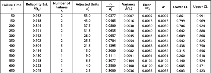
Once again, this type of problem is most readily solved by constructing a table similar to the following:

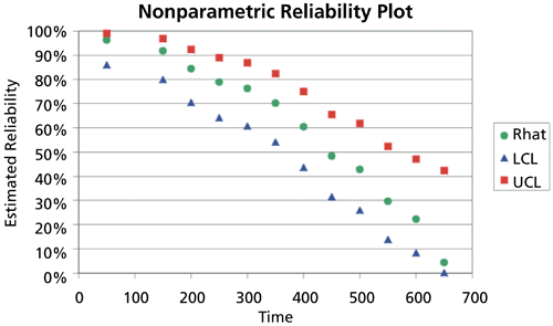
The following plot illustrates these results graphically: