Template:Mixed weibull confidence bounds

Mixed Weibull Confidence Bounds

In Weibull++, two methods are available for estimating the confidence bounds for the mixed Weibull distribution. The first method is the beta binomial, described in Confidence Bounds chapter. The second method is the Fisher matrix confidence bounds. For the Fisher matrix bounds, the methodology is the same as described in Confidence Bounds chapter. The variance/covariance matrix for the mixed Weibull is a [math]\displaystyle{ (3\cdot S-1)\times (3\cdot S-1) }[/math] matrix, where [math]\displaystyle{ S }[/math] is the number of subpopulations. Bounds on the parameters, reliability and time are estimated using the same transformations and methods that were used for the The Weibull Distribution chapter. Note, however, that in addition to the Weibull parameters, the bounds on the subpopulation portions are obtained as well. The bounds on the portions are estimated by:

[math]\displaystyle{ \begin{align} & {{\rho }_{U}}= & \frac{{\hat{\rho }}}{\hat{\rho }+(1-\hat{\rho }){{e}^{-\tfrac{{{K}_{\alpha }}\sqrt{Var(\widehat{\rho })}}{\hat{\rho }(1-\hat{\rho })}}}} \\ & & \\ & {{\rho }_{L}}= & \frac{{\hat{\rho }}}{\hat{\rho }+(1-\hat{\rho }){{e}^{\tfrac{{{K}_{\alpha }}\sqrt{Var(\widehat{\rho })}}{\hat{\rho }(1-\hat{\rho })}}}} \end{align} }[/math]

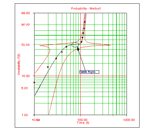
where [math]\displaystyle{ Var(\widehat{\rho }) }[/math] is obtained from the variance/covariance matrix. When using the Fisher matrix bounds method, problems can occur on the transition points of the distribution, and in particular on the Type 1 confidence bounds (bounds on time). The problems (i.e. the departure from the expected monotonic behavior) occur when the transition region between two subpopulations becomes a ``saddle (i.e. the probability line is almost parallel to the time axis on a probability plot). In this case, the bounds on time approach infinity. This behavior is more frequently encountered with smaller sample sizes. The physical interpretation is that there is insufficient data to support any inferences when in this region.

This is graphically illustrated in the following figure. In this plot it can be seen that there are no data points between the last point of the first subpopulation and the first point of the second subpopulation, thus the uncertainty is high, as described by the mathematical model.

Beta binomial bounds can be used instead in these cases, especially when estimations are to be obtained close to these regions.