The Mixed Weibull Distribution

Other Distributions

Besides the Weibull, exponential, normal and lognormal, there are other distributions that are used to model reliability and life data. However, these four represent the most prominent distributions in Weibull++. In this chapter, we will discuss other distributions that are used under special circumstances: the mixed Weibull, the generalized gamma, the Gumbel, the logistic and the loglogistic distributions.

Mixed Weibull Distribution

The mixed Weibull distribution (also known as a multimodal Weibull) is used to model data that do not fall on a straight line on a Weibull probability plot. Data of this type, particularly if the data points follow an S-shape on the probability plot, may be indicative of more than one failure mode at work in the population of failure times. Field data from a given mixed population may frequently represent multiple failure modes. The necessity of determining the life regions where these failure modes occur is apparent when it is realized that the times-to-failure for each mode may follow a distinct Weibull distribution, thus requiring individual mathematical treatment. Another reason is that each failure mode may require a different design change to improve the component's reliability [19].

A decreasing failure rate is usually encountered during the early life period of components when the substandard components fail and are removed from the population. The failure rate continues to decrease until all such substandard components fail and are removed. This corresponds to a decreasing failure rate. The Weibull distribution having [math]\displaystyle{ \beta \lt 1 }[/math] is often used to depict this life characteristic.

A second type of failure prevails when the components fail by chance alone and their failure rate is nearly constant. This can be caused by sudden, unpredictable stress applications that have a stress level above those to which the product is designed. Such failures tend to occur throughout the life of a component. The distributions most often used to describe this failure rate characteristic are the exponential distribution and the Weibull distribution with [math]\displaystyle{ \beta \approx 1 }[/math] .

A third type of failure is characterized by a failure rate that increases as operating hours are accumulated. Usually, wear has started to set in and this brings the component's performance out of specification. As age increases further, this wear-out process removes more and more components until all components fail. The normal distribution and the Weibull distribution with a [math]\displaystyle{ \beta \gt 1 }[/math] have been successfully used to model the times-to-failure distribution during the wear-out period.

Several different failure modes may occur during the various life periods. A methodology is needed to identify these failure modes and determine their failure distributions and reliabilities. This section presents a procedure whereby the proportion of units failing in each mode is determined and their contribution to the reliability of the component is quantified. From this reliability expression, the remaining major reliability functions, the probability density, the failure rate and the conditional-reliability functions are calculated to complete the reliability analysis of such mixed populations.

Background

Consider a life test of identical components. The components were placed in a test at age [math]\displaystyle{ T=0 }[/math] and were tested to failure, with their times-to-failure recorded. Further assume that the test covered the entire lifespan of the units, and different failure modes were observed over each region of life, namely early life (early failure mode), chance life (chance failure mode), and wear-out life (wear-out failure mode). Also, as items failed during the test, they were removed from the test, inspected and segregated into lots according to their failure mode. At the conclusion of the test, there will be [math]\displaystyle{ n }[/math] subpopulations of [math]\displaystyle{ {{N}_{1}},{{N}_{2}},{{N}_{3}},...,{{N}_{n}} }[/math] failed components. If the events of the test are now reconstructed, it may be theorized that at age [math]\displaystyle{ T=0 }[/math] there were actually [math]\displaystyle{ n }[/math] separate subpopulations in the test, each with a different times-to-failure distribution and failure mode, even though at [math]\displaystyle{ T=0 }[/math] the subpopulations were not physically distinguishable. The mixed Weibull methodology accomplishes this segregation based on the results of the life test.

If [math]\displaystyle{ N }[/math] identical components from a mixed population undertake a mission of [math]\displaystyle{ T }[/math] duration, starting the mission at age zero, then the number of components surviving this mission can be found from the following definition of reliability:

[math]\displaystyle{ {{R}_{1,2,...,n}}(T)=\frac{{{N}_{1,2,3,..,{{n}_{S}}}}(T)}{N} }[/math]

Then:

[math]\displaystyle{ \begin{align} {{N}_{1,2,...,{{n}_{S}}}}(T)= & N[{{R}_{1,2,...,n}}(T)] \\ \\ {{N}_{{{1}_{S}}}}(T)=& {{N}_{1}}{{R}_{1}}(T);{{N}_{{{2}_{S}}}}(T)={{N}_{2}}{{R}_{2}}(T) \\ {{N}_{{{3}_{S}}}}(T)=& {{N}_{3}}{{R}_{3}}(T);...;{{N}_{{{n}_{S}}}}={{N}_{n}}{{R}_{n}}(T) \end{align} }[/math]

The total number surviving by age [math]\displaystyle{ T }[/math] in the mixed population is the sum of the number surviving in all subpopulations or:

[math]\displaystyle{ {{N}_{1,2,...,{{n}_{S}}}}(T)={{N}_{{{1}_{S}}}}(T)+{{N}_{{{2}_{S}}}}(T)+{{N}_{{{3}_{S}}}}(T)+\cdots +{{N}_{{{n}_{S}}}}(T) }[/math]

Substituting into Eqn. (rel) yields:

[math]\displaystyle{ {{R}_{1,2,...,n}}(T)=\frac{1}{N}[{{N}_{1}}{{R}_{1}}(T)+{{N}_{2}}{{R}_{2}}(T)+{{N}_{3}}{{R}_{3}}(T)+\cdots +{{N}_{n}}{{R}_{n}}(T)] }[/math]

or:

[math]\displaystyle{ {{R}_{1,2,...,n}}(T)=\frac{{{N}_{1}}}{N}{{R}_{1}}(T)+\frac{{{N}_{2}}}{N}{{R}_{2}}(T)+\frac{{{N}_{3}}}{N}{{R}_{3}}(T)+\cdots +\frac{{{N}_{n}}}{N}{{R}_{n}}(T) }[/math]

This expression can also be derived by applying Bayes' theorem [20], which says that the reliability of a component drawn at random from a mixed population composed of [math]\displaystyle{ n }[/math] types of failure subpopulations is its reliability, [math]\displaystyle{ {{R}_{1}}(T) }[/math] , given that the component is from subpopulation 1, or [math]\displaystyle{ \tfrac{{{N}_{1}}}{N} }[/math] plus its reliability, [math]\displaystyle{ {{R}_{2}}(T) }[/math] , given that the component is from subpopulation 2, or [math]\displaystyle{ \tfrac{{{N}_{2}}}{N} }[/math] plus its reliability, [math]\displaystyle{ {{R}_{3}}(T) }[/math] , given that the component is from subpopulation 3, or [math]\displaystyle{ \tfrac{{{N}_{3}}}{N} }[/math] , and so on, plus its reliability, [math]\displaystyle{ {{R}_{n}}(T) }[/math] , given that the component is from subpopulation [math]\displaystyle{ n }[/math] , or [math]\displaystyle{ \tfrac{{{N}_{n}}}{N} }[/math] , and:

[math]\displaystyle{ \underset{i=1}{\overset{n}{\mathop \sum }}\,\frac{{{N}_{i}}}{N}=1 }[/math]

This may be written mathematically as:

[math]\displaystyle{ {{R}_{1,2,...,n}}(T)=\frac{{{N}_{1}}}{N}{{R}_{1}}(T)+\frac{{{N}_{2}}}{N}{{R}_{2}}(T)+\frac{{{N}_{3}}}{N}{{R}_{3}}(T)+\cdots +\frac{{{N}_{n}}}{N}{{R}_{n}}(T) }[/math]

Other functions of reliability engineering interest are found by applying the fundamentals to Eqn. (rel1).

For example, the probability density function can be found from:

[math]\displaystyle{ \begin{align} {{f}_{1,2,...,n}}(T)= & -\frac{d}{dT}[{{R}_{1,2,...,n}}(T)] \\ {{f}_{1,2,...,n}}(T)= & \frac{{{N}_{1}}}{N}\left( -\frac{d}{dT}[{{R}_{1}}(T)] \right)+\frac{{{N}_{2}}}{N}\left( -\frac{d}{dT}[{{R}_{2}}(T)] \right) \\ & +\ \ \frac{{{N}_{3}}}{N}\left( -\frac{d}{dT}[{{R}_{3}}(T)] \right)+\cdots +\frac{{{N}_{n}}}{N}\left( -\frac{d}{dT}[{{R}_{n}}(T)] \right) \\ {{f}_{1,2,...,n}}(T)= & \frac{{{N}_{1}}}{N}{{f}_{1}}(T)+\frac{{{N}_{2}}}{N}{{f}_{2}}(T) \\ & +\ \ \frac{{{N}_{3}}}{N}{{f}_{3}}(T)+\cdots +\frac{{{N}_{n}}}{N}{{f}_{n}}(T) \end{align} }[/math]

Also, the failure rate function of a population is given by:

[math]\displaystyle{ \begin{align} {{\lambda }_{1,2,...,n}}(T)= & \frac{{{f}_{1,2,...,n}}(T)}{{{R}_{1,2,...,n}}(T)}, \\ {{\lambda }_{1,2,...,n}}(T)= & \frac{\tfrac{{{N}_{1}}}{N}{{f}_{1}}(T)+\tfrac{{{N}_{2}}}{N}{{f}_{2}}(T)+\tfrac{{{N}_{3}}}{N}{{f}_{3}}(T)+\cdots +\tfrac{{{N}_{n}}}{N}{{f}_{n}}(T)}{\tfrac{{{N}_{1}}}{N}{{R}_{1}}(T)+\tfrac{{{N}_{2}}}{N}{{R}_{2}}(T)+\tfrac{{{N}_{3}}}{N}{{R}_{3}}(T)+\cdots +\tfrac{{{N}_{n}}}{N}{{R}_{n}}(T)}. \end{align} }[/math]

The conditional reliability for a new mission of duration [math]\displaystyle{ t }[/math] , starting this mission at age [math]\displaystyle{ T }[/math] , or after having already operated a total of [math]\displaystyle{ T }[/math] hours, is given by:

[math]\displaystyle{ \begin{align} {{R}_{1,2,...,n}}(T,t)= & \frac{{{R}_{1,2,...,n}}(T+t)}{{{R}_{1,2,...,n}}(T)} \\ {{R}_{1,2,...,n}}(T,t)= & \frac{\tfrac{{{N}_{1}}}{N}{{R}_{1}}(T+t)+\tfrac{{{N}_{2}}}{N}{{R}_{2}}(T+t)+\cdots +\tfrac{{{N}_{n}}}{N}{{R}_{n}}(T+t)}{\tfrac{{{N}_{1}}}{N}{{R}_{1}}(T)+\tfrac{{{N}_{2}}}{N}{{R}_{2}}(T)+\cdots +\tfrac{{{N}_{n}}}{N}{{R}_{n}}(T)} \end{align} }[/math]

The Mixed Weibull Equations

Depending on the number of subpopulations chosen, Weibull++ uses the following equations for the reliability and probability density functions:

[math]\displaystyle{ {{R}_{1,...,S}}(T)=\underset{i=1}{\overset{S}{\mathop \sum }}\,\frac{{{N}_{i}}}{N}{{e}^{-{{\left( \tfrac{T}{{{\eta }_{i}}} \right)}^{{{\beta }_{i}}}}}} }[/math]

and:

[math]\displaystyle{ {{f}_{1,...,S}}(T)=\underset{i=1}{\overset{S}{\mathop \sum }}\,\frac{{{N}_{i}}{{\beta }_{i}}}{N{{\eta }_{i}}}{{\left( \frac{T}{{{\eta }_{i}}} \right)}^{{{\beta }_{i}}-1}}{{e}^{-{{(\tfrac{T}{{{\eta }_{i}}})}^{{{\beta }_{i}}}}}} }[/math]

where [math]\displaystyle{ S=2 }[/math] , [math]\displaystyle{ S=3 }[/math] , and [math]\displaystyle{ S=4 }[/math] for 2, 3 and 4 subpopulations respectively. Weibull++ uses a non-linear regression method or direct maximum likelihood methods to estimate the parameters.

Mixed Weibull Parameter Estimation

Regression Solution

Weibull++ utilizes a modified Levenberg-Marquardt algorithm (non-linear regression) when performing regression analysis on a mixed Weibull distribution. The procedure is rather involved and is beyond the scope of this reference. It is sufficient to say that the algorithm fits a curved line of the form:

[math]\displaystyle{ {{R}_{1,...,S}}(T)=\underset{i=1}{\overset{S}{\mathop \sum }}\,{{\rho }_{i}}\cdot {{e}^{-{{\left( \tfrac{T}{{{\eta }_{i}}} \right)}^{{{\beta }_{i}}}}}} }[/math]

where:

[math]\displaystyle{ \underset{i=1}{\overset{S}{\mathop \sum }}\,{{\rho }_{i}}=1 }[/math]

to the parameters [math]\displaystyle{ \widehat{{{\rho }_{1,\text{ }}}} }[/math] [math]\displaystyle{ \widehat{{{\beta }_{1}}}, }[/math] [math]\displaystyle{ \widehat{{{\eta }_{1}}}, }[/math] [math]\displaystyle{ \widehat{{{\rho }_{2,\text{ }}}}\widehat{{{\beta }_{2}}}, }[/math] [math]\displaystyle{ \widehat{{{\eta }_{2}}},..., }[/math] [math]\displaystyle{ \widehat{{{\rho }_{S,}}\text{ }}\widehat{{{\beta }_{S}}}, }[/math] [math]\displaystyle{ \widehat{{{\eta }_{S}}}, }[/math] utilizing the times-to-failure and their respective plotting positions. It is important to note that in the case of regression analysis, using a mixed Weibull model, the choice of regression axis, i.e. [math]\displaystyle{ RRX }[/math] or [math]\displaystyle{ RRY, }[/math] is of no consequence since non-linear regression is utilized.

MLE

The same space of parameters, namely [math]\displaystyle{ \widehat{{{\rho }_{1,\text{ }}}} }[/math] [math]\displaystyle{ \widehat{{{\beta }_{1}}}, }[/math] [math]\displaystyle{ \widehat{{{\eta }_{1}}}, }[/math] [math]\displaystyle{ \widehat{{{\rho }_{2,\text{ }}}}\widehat{{{\beta }_{2}}}, }[/math] [math]\displaystyle{ \widehat{{{\eta }_{2}}},..., }[/math] [math]\displaystyle{ \widehat{{{\rho }_{S,}}\text{ }}\widehat{{{\beta }_{S}}}, }[/math] [math]\displaystyle{ \widehat{{{\eta }_{S}}}, }[/math] is also used under the MLE method, using the likelihood function as given in Appendix C of this reference. Weibull++ uses the EM algorithm, short for Expectation-Maximization algorithm, for the MLE analysis. Details on the numerical procedure are beyond the scope of this reference.

Mixed Weibull Confidence Bounds

In Weibull++, two methods are available for estimating the confidence bounds for the mixed Weibull distribution. The first method is the beta binomial, described in Chapter 5. The second method is the Fisher matrix confidence bounds. For the Fisher matrix bounds, the methodology is the same as described in Chapter 5. The variance/covariance matrix for the mixed Weibull is a [math]\displaystyle{ (3\cdot S-1)\times (3\cdot S-1) }[/math] matrix, where [math]\displaystyle{ S }[/math] is the number of subpopulations. Bounds on the parameters, reliability and time are estimated using the same transformations and methods that were used for the Weibull distribution (Chapter 6). Note, however, that in addition to the Weibull parameters, the bounds on the subpopulation portions are obtained as well. The bounds on the portions are estimated by:

[math]\displaystyle{ \begin{align} & {{\rho }_{U}}= & \frac{{\hat{\rho }}}{\hat{\rho }+(1-\hat{\rho }){{e}^{-\tfrac{{{K}_{\alpha }}\sqrt{Var(\widehat{\rho })}}{\hat{\rho }(1-\hat{\rho })}}}} \\ & & \\ & {{\rho }_{L}}= & \frac{{\hat{\rho }}}{\hat{\rho }+(1-\hat{\rho }){{e}^{\tfrac{{{K}_{\alpha }}\sqrt{Var(\widehat{\rho })}}{\hat{\rho }(1-\hat{\rho })}}}} \end{align} }[/math]

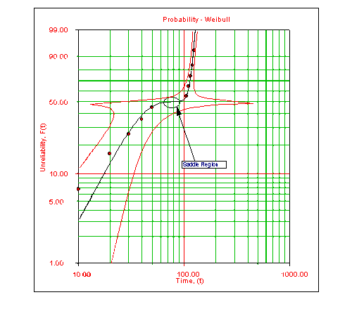
where [math]\displaystyle{ Var(\widehat{\rho }) }[/math] is obtained from the variance/covariance matrix. When using the Fisher matrix bounds method, problems can occur on the transition points of the distribution, and in particular on the Type 1 confidence bounds (bounds on time). The problems (i.e. the departure from the expected monotonic behavior) occur when the transition region between two subpopulations becomes a ``saddle (i.e. the probability line is almost parallel to the time axis on a probability plot). In this case, the bounds on time approach infinity. This behavior is more frequently encountered with smaller sample sizes. The physical interpretation is that there is insufficient data to support any inferences when in this region.

This is graphically illustrated in the following figure. In this plot it can be seen that there are no data points between the last point of the first subpopulation and the first point of the second subpopulation, thus the uncertainty is high, as described by the mathematical model.

Beta binomial bounds can be used instead in these cases, especially when estimations are to be obtained close to these regions.

Using the Mixed Weibull Distribution in Weibull++

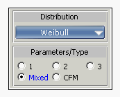
To use the mixed Weibull distribution, simply select the Mixed option under Parameters/Type, and click the Calculate icon. A window will appear asking you which form of the mixed Weibull you would like to use, i.e. S = 2, 3 or 4. In other words, How many subpopulations would you like to consider?

Simply select the number of subpopulations you would like to consider and click OK. The application will automatically calculate the parameters of each subpopulation for you.

Viewing the Calculated Parameters

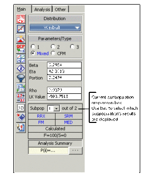
When using the Mixed Weibull option, the parameters given in the result area apply to different subpopulations. To view the results for a particular subpopulation, select the subpopulation, as shown next.

About the Calculated Parameters

Weibull++ uses the numbers 1, 2, 3 and 4 (or first, second, third and fourth subpopulation) to identify each subpopulation. These are just designations for each subpopulation, and they are ordered based on the value of the scale parameter, [math]\displaystyle{ \eta }[/math] . Since the equation used is additive or:

[math]\displaystyle{ {{R}_{1,..,S}}(T)=\underset{i=1}{\overset{S}{\mathop \sum }}\,\frac{{{N}_{i}}}{N}{{e}^{-{{\left( \tfrac{T}{{{\eta }_{i}}} \right)}^{{{\beta }_{i}}}}}} }[/math]

the order of the subpopulations which are given the designation 1, 2, 3, or 4 is of no consequence. For consistency, the application will always return the order of the results based on the magnitude of the scale parameter.

Mixed Weibull, Other Uses

Reliability Bathtub Curves

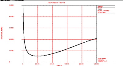
A reliability bathtub curve is nothing more than the graph of the failure rate versus time, over the life of the product. In general, the life stages of the product consist of early, chance and wear-out. Weibull++ allows you to plot this by simply selecting the failure rate plot, as shown next.

Determination of the Burn-in Period

If the failure rate goal is known, then the burn-in period can be found from the failure rate plot by drawing a horizontal line at the failure rate goal level and then finding the intersection with the failure rate curve. Next, drop vertically at the intersection, and read off the burn-in time from the time axis. This burn-in time helps insure that the population will have a failure rate that is at least equal to or lower than the goal after the burn-in period. The same could also be obtained using the Function Wizard and generating different failure rates based on time increments. Using these generated times and the corresponding failure rates, one can decide on the optimum burn-in time versus the corresponding desired failure rate.

A Mixed Weibull Example

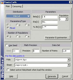
We will illustrate mixed Weibull analysis using a Monte Carlo generated set of data. To repeat this example, generate data from a two-parameter Weibull distribution, using the Weibull++ Monte Carlo data window. The following figures illustrate the required steps, inputs and results.

• In the Monte Carlo window, enter the values and select the options shown below for subpopulation 1.

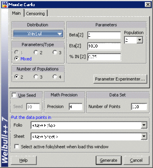
Switch to subpopulation 2 and make the selection shown below. Click Generate.

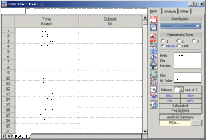
• After the data has been generated, choose the Weibull distribution and select Mixed for the Parameters/Type. Click the Calculate icon and then choose Two (2) Population Weibull Analysis. Click OK.

The results for subpopulation 1 are shown next. (Note that your results could be different due to the randomness of the simulation.)

The results for subpopulation 2 are shown next (Note that your results could be different due to the randomness of the simulation.)

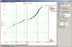
The Weibull probability plot for this data is shown next (Note that your results could be different due to the randomness of the simulation.)