The Lognormal Distribution: Difference between revisions
| Line 134: | Line 134: | ||
::<math>F({T}')=\Phi \left( \frac{{T}'-{\mu }'}{{{\sigma }_{{{T}'}}}} \right)</math> | ::<math>F({T}')=\Phi \left( \frac{{T}'-{\mu }'}{{{\sigma }_{{{T}'}}}} \right)</math> | ||
:or: | |||
or: | |||
::<math>{{\Phi }^{-1}}\left[ F({T}') \right]=-\frac{{{\mu }'}}{{{\sigma }_{{{T}'}}}}+\frac{1}{{{\sigma }_{{{T}'}}}}\cdot {T}'</math> | ::<math>{{\Phi }^{-1}}\left[ F({T}') \right]=-\frac{{{\mu }'}}{{{\sigma }_{{{T}'}}}}+\frac{1}{{{\sigma }_{{{T}'}}}}\cdot {T}'</math> | ||
:where: | |||
where: | |||
::<math>\Phi (x)=\frac{1}{\sqrt{2\pi }}\int_{-\infty }^{x}{{e}^{-\tfrac{{{t}^{2}}}{2}}}dx</math> | ::<math>\Phi (x)=\frac{1}{\sqrt{2\pi }}\int_{-\infty }^{x}{{e}^{-\tfrac{{{t}^{2}}}{2}}}dx</math> | ||
:Now, let: | |||
Now, let: | |||
::<math>y={{\Phi }^{-1}}\left[ F({T}') \right]</math> | ::<math>y={{\Phi }^{-1}}\left[ F({T}') \right]</math> | ||
::<math>a=-\frac{{{\mu }'}}{{{\sigma }_{{{T}'}}}}</math> | ::<math>a=-\frac{{{\mu }'}}{{{\sigma }_{{{T}'}}}}</math> | ||
:and: | |||
and: | |||
::<math>b=\frac{1}{{{\sigma }_{{{T}'}}}}</math> | ::<math>b=\frac{1}{{{\sigma }_{{{T}'}}}}</math> | ||
which results in the linear equation of: | which results in the linear equation of: | ||
| Line 177: | Line 169: | ||
=====Solution to Example 1===== | =====Solution to Example 1===== | ||
In order to plot the points for the probability plot, the appropriate unreliability estimate values must be obtained. These will be estimated through the use of median ranks, which can be obtained from statistical tables or the Quick Statistical Reference in Weibull++. The following table shows the times-to-failure and the appropriate median rank values for this example: | In order to plot the points for the probability plot, the appropriate unreliability estimate values must be obtained. These will be estimated through the use of median ranks, which can be obtained from statistical tables or the Quick Statistical Reference in Weibull++. The following table shows the times-to-failure and the appropriate median rank values for this example: | ||
<center><math>\begin{matrix} | <center><math>\begin{matrix} | ||
| Line 191: | Line 182: | ||
\text{9000} & \text{91}\text{.70 }\!\!%\!\!\text{ } \\ | \text{9000} & \text{91}\text{.70 }\!\!%\!\!\text{ } \\ | ||
\end{matrix}</math></center> | \end{matrix}</math></center> | ||
Revision as of 19:03, 19 August 2011
The Lognormal Distribution
The lognormal distribution is commonly used to model the lives of units whose failure modes are of a fatigue-stress nature. Since this includes most, if not all, mechanical systems, the lognormal distribution can have widespread application. Consequently, the lognormal distribution is a good companion to the Weibull distribution when attempting to model these types of units. As may be surmised by the name, the lognormal distribution has certain similarities to the normal distribution. A random variable is lognormally distributed if the logarithm of the random variable is normally distributed. Because of this, there are many mathematical similarities between the two distributions. For example, the mathematical reasoning for the construction of the probability plotting scales and the bias of parameter estimators is very similar for these two distributions.
Lognormal Probability Density Function
The lognormal distribution is a two-parameter distribution with parameters [math]\displaystyle{ {\mu }' }[/math] and [math]\displaystyle{ {{\sigma }_{{{T}'}}} }[/math] . The [math]\displaystyle{ pdf }[/math] for this distribution is given by:
- [math]\displaystyle{ f({T}')=\frac{1}{{{\sigma }_{{{T}'}}}\sqrt{2\pi }}{{e}^{-\tfrac{1}{2}{{\left( \tfrac{{{T}^{\prime }}-{\mu }'}{{{\sigma }_{{{T}'}}}} \right)}^{2}}}} }[/math]
where, [math]\displaystyle{ {T}'=\ln (T) }[/math]. , where the [math]\displaystyle{ T }[/math] values are the times-to-failure, and
- [math]\displaystyle{ \mu'=\text{mean of the natural logarithms} }[/math]
- [math]\displaystyle{ \text{of the times-to-failure,} }[/math]
- [math]\displaystyle{ \sigma_{T'}=\text{standard deviation of the natural logarithms} }[/math]
- [math]\displaystyle{ \text{of the times-to-failure} }[/math]
The lognormal [math]\displaystyle{ pdf }[/math] can be obtained, realizing that for equal probabilities under the normal and lognormal [math]\displaystyle{ pdf }[/math] s, incremental areas should also be equal, or:
- [math]\displaystyle{ f(T)dT=f({T}')d{T}' }[/math]
Taking the derivative yields:
- [math]\displaystyle{ d{T}'=\frac{dT}{T} }[/math]
- Substitution yields:
- [math]\displaystyle{ \begin{align} f(T)= & \frac{f({T}')}{T}, \\ f(T)= & \frac{1}{T\cdot {{\sigma }_{{{T}'}}}\sqrt{2\pi }}{{e}^{-\tfrac{1}{2}{{\left( \tfrac{\text{ln}(T)-{\mu }'}{{{\sigma }_{{{T}'}}}} \right)}^{2}}}} \end{align} }[/math]
- where:
- [math]\displaystyle{ f(T)\ge 0,T\gt 0,-\infty \lt {\mu }'\lt \infty ,{{\sigma }_{{{T}'}}}\gt 0 }[/math]
Lognormal Statistical Properties
The Mean or MTTF
The mean of the lognormal distribution, [math]\displaystyle{ \mu }[/math] , is given by [18]:
- [math]\displaystyle{ \mu ={{e}^{{\mu }'+\tfrac{1}{2}\sigma _{{{T}'}}^{2}}} }[/math]
The mean of the natural logarithms of the times-to-failure, [math]\displaystyle{ \mu' }[/math] , in terms of [math]\displaystyle{ \bar{T} }[/math] and [math]\displaystyle{ {{\sigma }_{T}} }[/math] is givgen by:
- [math]\displaystyle{ {\mu }'=\ln \left( {\bar{T}} \right)-\frac{1}{2}\ln \left( \frac{\sigma _{T}^{2}}{{{{\bar{T}}}^{2}}}+1 \right) }[/math]
The Median
The median of the lognormal distribution, [math]\displaystyle{ \breve{T} }[/math] , is given by [18]:
- [math]\displaystyle{ \breve{T}={{e}^{{{\mu }'}}} }[/math]
The Mode
The mode of the lognormal distribution, [math]\displaystyle{ \tilde{T} }[/math] , is given by [1]:
- [math]\displaystyle{ \tilde{T}={{e}^{{\mu }'-\sigma _{{{T}'}}^{2}}} }[/math]
The Standard Deviation
The standard deviation of the lognormal distribution, [math]\displaystyle{ {{\sigma }_{T}} }[/math] , is given by [18]:
- [math]\displaystyle{ {{\sigma }_{T}}=\sqrt{\left( {{e}^{2{\mu }'+\sigma _{{{T}'}}^{2}}} \right)\left( {{e}^{\sigma _{{{T}'}}^{2}}}-1 \right)} }[/math]
The standard deviation of the natural logarithms of the times-to-failure, [math]\displaystyle{ {{\sigma }_{{{T}'}}} }[/math] , in terms of [math]\displaystyle{ \bar{T} }[/math] and [math]\displaystyle{ {{\sigma }_{T}} }[/math] is given by:
- [math]\displaystyle{ {{\sigma }_{{{T}'}}}=\sqrt{\ln \left( \frac{\sigma _{T}^{2}}{{{{\bar{T}}}^{2}}}+1 \right)} }[/math]
The Lognormal Reliability Function
The reliability for a mission of time [math]\displaystyle{ T }[/math] , starting at age 0, for the lognormal distribution is determined by:
- [math]\displaystyle{ R(T)=\int_{T}^{\infty }f(t)dt }[/math]
- or:
- [math]\displaystyle{ R(T)=\int_{{{T}^{^{\prime }}}}^{\infty }\frac{1}{{{\sigma }_{{{T}'}}}\sqrt{2\pi }}{{e}^{-\tfrac{1}{2}{{\left( \tfrac{t-{\mu }'}{{{\sigma }_{{{T}'}}}} \right)}^{2}}}}dt }[/math]
As with the normal distribution, there is no closed-form solution for the lognormal reliability function. Solutions can be obtained via the use of standard normal tables. Since the application automatically solves for the reliability we will not discuss manual solution methods. For interested readers, full explanations can be found in the references.
The Lognormal Conditional Reliability
The lognormal conditional reliability function is given by:
- [math]\displaystyle{ R(t|T)=\frac{R(T+t)}{R(T)}=\frac{\int_{\text{ln}(T+t)}^{\infty }\tfrac{1}{{{\sigma }_{{{T}'}}}\sqrt{2\pi }}{{e}^{-\tfrac{1}{2}{{\left( \tfrac{s-{\mu }'}{{{\sigma }_{{{T}'}}}} \right)}^{2}}}}ds}{\int_{\text{ln}(T)}^{\infty }\tfrac{1}{{{\sigma }_{{{T}'}}}\sqrt{2\pi }}{{e}^{-\tfrac{1}{2}{{\left( \tfrac{s-{\mu }'}{{{\sigma }_{{{T}'}}}} \right)}^{2}}}}ds} }[/math]
Once again, the use of standard normal tables is necessary to solve this equation, as no closed-form solution exists.
The Lognormal Reliable Life
As there is no closed-form solution for the lognormal reliability equation, no closed-form solution exists for the lognormal reliable life either. In order to determine this value, one must solve the equation:
- [math]\displaystyle{ {{R}_{T}}=\int_{\text{ln}(T)}^{\infty }\frac{1}{{{\sigma }_{{{T}'}}}\sqrt{2\pi }}{{e}^{-\tfrac{1}{2}{{\left( \tfrac{s-{\mu }'}{{{\sigma }_{{{T}'}}}} \right)}^{2}}}}ds }[/math]
for [math]\displaystyle{ T }[/math] .
The Lognormal Failure Rate Function
The lognormal failure rate is given by:
- [math]\displaystyle{ \lambda (T)=\frac{f(T)}{R(T)}=\frac{\tfrac{1}{T\cdot {{\sigma }_{{{T}'}}}\sqrt{2\pi }}{{e}^{-\tfrac{1}{2}{{(\tfrac{{T}'-{\mu }'}{{{\sigma }_{{{T}'}}}})}^{2}}}}}{\int_{{{T}'}}^{\infty }\tfrac{1}{{{\sigma }_{{{T}'}}}\sqrt{2\pi }}{{e}^{-\tfrac{1}{2}{{(\tfrac{t-{\mu }'}{{{\sigma }_{{{T}'}}}})}^{2}}}}dt} }[/math]
As with the reliability equations, standard normal tables will be required to solve for this function.
Distribution Characteristics
[math]\displaystyle{ }[/math]
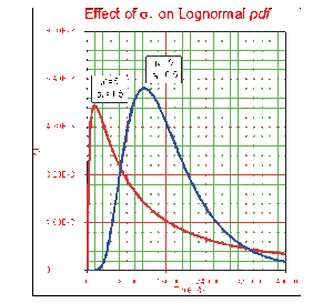
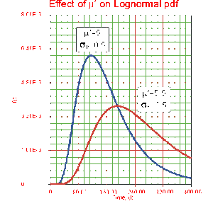
- • The lognormal distribution is a distribution skewed to the right.
- • The [math]\displaystyle{ pdf }[/math] starts at zero, increases to its mode, and decreases thereafter.
- • The degree of skewness increases as [math]\displaystyle{ {{\sigma }_{{{T}'}}} }[/math] increases, for a given [math]\displaystyle{ \mu' }[/math]
- • For the same [math]\displaystyle{ {{\sigma }_{{{T}'}}} }[/math] , the [math]\displaystyle{ pdf }[/math] 's skewness increases as [math]\displaystyle{ {\mu }' }[/math] increases.
- • For [math]\displaystyle{ {{\sigma }_{{{T}'}}} }[/math] values significantly greater than 1, the [math]\displaystyle{ pdf }[/math] rises very sharply in the beginning, i.e. for very small values of [math]\displaystyle{ T }[/math] near zero, and essentially follows the ordinate axis, peaks out early, and then decreases sharply like an exponential [math]\displaystyle{ pdf }[/math] or a Weibull [math]\displaystyle{ pdf }[/math] with [math]\displaystyle{ 0\lt \beta \lt 1 }[/math] .
- • The parameter, [math]\displaystyle{ {\mu }' }[/math], in terms of the logarithm of the [math]\displaystyle{ {T}'s }[/math] is also the scale parameter, and not the location parameter as in the case of the normal [math]\displaystyle{ pdf }[/math] .
- • The parameter [math]\displaystyle{ {{\sigma }_{{{T}'}}} }[/math], or the standard deviation of the [math]\displaystyle{ {T}'s }[/math] in terms of their logarithm or of their [math]\displaystyle{ {T}' }[/math], is also the shape parameter and not the scale parameter, as in the normal [math]\displaystyle{ pdf }[/math], and assumes only positive values.
Lognormal Distribution Parameters in Weibull++
In Weibull++, the parameters returned for the lognormal distribution are always logarithmic. That is: the parameter [math]\displaystyle{ {\mu }' }[/math] represents the mean of the natural logarithms of the times-to-failure, while [math]\displaystyle{ {{\sigma }_{{{T}'}}} }[/math] represents the standard deviation of these data point logarithms. Specifically, the returned [math]\displaystyle{ {{\sigma }_{{{T}'}}} }[/math] is the square root of the variance of the natural logarithms of the data points. Even though the application denotes these values as mean and standard deviation, the user is reminded that these are given as the parameters of the distribution, and are thus the mean and standard deviation of the natural logarithms of the data. The mean value of the times-to-failure, not used as a parameter, as well as the standard deviation can be obtained through the QCP or the Function Wizard.
Estimation of the Parameters
Probability Plotting
As described before, probability plotting involves plotting the failure times and associated unreliability estimates on specially constructed probability plotting paper. The form of this paper is based on a linearization of the [math]\displaystyle{ cdf }[/math] of the specific distribution. For the lognormal distribution, the cumulative density function can be written as:
- [math]\displaystyle{ F({T}')=\Phi \left( \frac{{T}'-{\mu }'}{{{\sigma }_{{{T}'}}}} \right) }[/math]
- or:
- [math]\displaystyle{ {{\Phi }^{-1}}\left[ F({T}') \right]=-\frac{{{\mu }'}}{{{\sigma }_{{{T}'}}}}+\frac{1}{{{\sigma }_{{{T}'}}}}\cdot {T}' }[/math]
- where:
- [math]\displaystyle{ \Phi (x)=\frac{1}{\sqrt{2\pi }}\int_{-\infty }^{x}{{e}^{-\tfrac{{{t}^{2}}}{2}}}dx }[/math]
- Now, let:
- [math]\displaystyle{ y={{\Phi }^{-1}}\left[ F({T}') \right] }[/math]
- [math]\displaystyle{ a=-\frac{{{\mu }'}}{{{\sigma }_{{{T}'}}}} }[/math]
- and:
- [math]\displaystyle{ b=\frac{1}{{{\sigma }_{{{T}'}}}} }[/math]
which results in the linear equation of:
- [math]\displaystyle{ y=a+b{T}' }[/math]
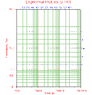
The normal probability paper resulting from this linearized [math]\displaystyle{ cdf }[/math] function is shown next.
The process for reading the parameter estimate values from the lognormal probability plot is very similar to the method employed for the normal distribution (see Chapter 8). However, since the lognormal distribution models the natural logarithms of the times-to-failure, the values of the parameter estimates must be read and calculated based on a logarithmic scale, as opposed to the linear time scale as it was done with the normal distribution. This parameter scale appears at the top of the lognormal probability plot.
The process of lognormal probability plotting is illustrated in the following example.
Example 1
Eight units are put on a life test and tested to failure. The failures occurred at 45, 140, 260, 500, 850, 1400, 3000, and 9000 hours. Estimate the parameters for the lognormal distribution using probability plotting.
Solution to Example 1
In order to plot the points for the probability plot, the appropriate unreliability estimate values must be obtained. These will be estimated through the use of median ranks, which can be obtained from statistical tables or the Quick Statistical Reference in Weibull++. The following table shows the times-to-failure and the appropriate median rank values for this example:
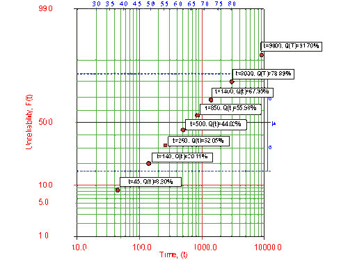
These points may now be plotted on normal probability plotting paper as shown in the next figure.
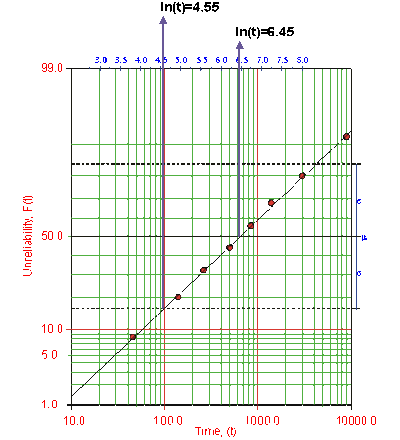
Draw the best possible line through the plot points. The time values where this line intersects the 15.85% and 50% unreliability values should be projected up to the logarithmic scale, as shown in the following plot.
The natural logarithm of the time where the fitted line intersects .. is equivalent to [math]\displaystyle{ {\mu }' }[/math] . In this case, [math]\displaystyle{ {\mu }'=6.45 }[/math] . The value for [math]\displaystyle{ {{\sigma }_{{{T}'}}} }[/math] is equal to the difference between the natural logarithms of the times where the fitted line crosses [math]\displaystyle{ Q(t)=50% }[/math] and [math]\displaystyle{ Q(t)=15.85%. }[/math] At [math]\displaystyle{ Q(t)=15.85% }[/math] , ln [math]\displaystyle{ (t)=4.55 }[/math] . Therefore, [math]\displaystyle{ {{\sigma }_{{{T}'}}}=6.45-4.55=1.9 }[/math] .
Rank Regression on Y
Performing a rank regression on Y requires that a straight line be fitted to a set of data points such that the sum of the squares of the vertical deviations from the points to the line is minimized.
The least squares parameter estimation method, or regression analysis, was discussed in Chapter 3 and the following equations for regression on Y were derived, and are again applicable:
- [math]\displaystyle{ \hat{a}=\bar{y}-\hat{b}\bar{x}=\frac{\underset{i=1}{\overset{N}{\mathop{\sum }}}\,{{y}_{i}}}{N}-\hat{b}\frac{\underset{i=1}{\overset{N}{\mathop{\sum }}}\,{{x}_{i}}}{N} }[/math]
and:
- [math]\displaystyle{ \hat{b}=\frac{\underset{i=1}{\overset{N}{\mathop{\sum }}}\,{{x}_{i}}{{y}_{i}}-\tfrac{\underset{i=1}{\overset{N}{\mathop{\sum }}}\,{{x}_{i}}\underset{i=1}{\overset{N}{\mathop{\sum }}}\,{{y}_{i}}}{N}}{\underset{i=1}{\overset{N}{\mathop{\sum }}}\,x_{i}^{2}-\tfrac{{{\left( \underset{i=1}{\overset{N}{\mathop{\sum }}}\,{{x}_{i}} \right)}^{2}}}{N}} }[/math]
In our case the equations for [math]\displaystyle{ {{y}_{i}} }[/math] and [math]\displaystyle{ x_{i} }[/math] are:
- [math]\displaystyle{ {{y}_{i}}={{\Phi }^{-1}}\left[ F(T_{i}^{\prime }) \right] }[/math]
and:
- [math]\displaystyle{ {{x}_{i}}=T_{i}^{\prime } }[/math]
where the [math]\displaystyle{ F(T_{i}^{\prime }) }[/math] is estimated from the median ranks. Once [math]\displaystyle{ \widehat{a} }[/math] and [math]\displaystyle{ \widehat{b} }[/math] are obtained, then [math]\displaystyle{ \widehat{\sigma } }[/math] and [math]\displaystyle{ \widehat{\mu } }[/math] can easily be obtained from Eqns. (aln) and (bln).
The Correlation Coefficient
The estimator of [math]\displaystyle{ \rho }[/math] is the sample correlation coefficient, [math]\displaystyle{ \hat{\rho } }[/math] , given by:
- [math]\displaystyle{ \hat{\rho }=\frac{\underset{i=1}{\overset{N}{\mathop{\sum }}}\,({{x}_{i}}-\overline{x})({{y}_{i}}-\overline{y})}{\sqrt{\underset{i=1}{\overset{N}{\mathop{\sum }}}\,{{({{x}_{i}}-\overline{x})}^{2}}\cdot \underset{i=1}{\overset{N}{\mathop{\sum }}}\,{{({{y}_{i}}-\overline{y})}^{2}}}} }[/math]
Example 2
Fourteen units were reliability tested and the following life test data were obtained:
| Table 9.1 - Life Test Data for Example 2 | |
| Data point index | Time-to-failure |
| 1 | 5 |
| 2 | 10 |
| 3 | 15 |
| 4 | 20 |
| 5 | 25 |
| 6 | 30 |
| 7 | 35 |
| 8 | 40 |
| 9 | 50 |
| 10 | 60 |
| 11 | 70 |
| 12 | 80 |
| 13 | 90 |
| 14 | 100 |
Assuming the data follow a lognormal distribution, estimate the parameters and the correlation coefficient, [math]\displaystyle{ \rho }[/math] , using rank regression on Y.
Solution to Example 2
Construct Table 9.2, as shown next.
The median rank values ( [math]\displaystyle{ F({{T}_{i}}) }[/math] ) can be found in rank tables or by using the Quick Statistical Reference in Weibull++ .
The [math]\displaystyle{ {{y}_{i}} }[/math] values were obtained from the standardized normal distribution's area tables by entering for [math]\displaystyle{ F(z) }[/math] and getting the corresponding [math]\displaystyle{ z }[/math] value ( [math]\displaystyle{ {{y}_{i}} }[/math] ). Given the values in the table above, calculate [math]\displaystyle{ \widehat{a} }[/math] and [math]\displaystyle{ \widehat{b} }[/math] using Eqns. (aaln) and (bbln):
- [math]\displaystyle{ \begin{align} & \widehat{b}= & \frac{\underset{i=1}{\overset{14}{\mathop{\sum }}}\,T_{i}^{\prime }{{y}_{i}}-(\underset{i=1}{\overset{14}{\mathop{\sum }}}\,T_{i}^{\prime })(\underset{i=1}{\overset{14}{\mathop{\sum }}}\,{{y}_{i}})/14}{\underset{i=1}{\overset{14}{\mathop{\sum }}}\,T_{i}^{\prime 2}-{{(\underset{i=1}{\overset{14}{\mathop{\sum }}}\,T_{i}^{\prime })}^{2}}/14} \\ & & \\ & \widehat{b}= & \frac{10.4473-(49.2220)(0)/14}{183.1530-{{(49.2220)}^{2}}/14} \end{align} }[/math]
or:
- [math]\displaystyle{ \widehat{b}=1.0349 }[/math]
and:
- [math]\displaystyle{ \widehat{a}=\frac{\underset{i=1}{\overset{N}{\mathop{\sum }}}\,{{y}_{i}}}{N}-\widehat{b}\frac{\underset{i=1}{\overset{N}{\mathop{\sum }}}\,T_{i}^{\prime }}{N} }[/math]
or:
- [math]\displaystyle{ \widehat{a}=\frac{0}{14}-(1.0349)\frac{49.2220}{14}=-3.6386 }[/math]
Therefore, from Eqn. (bln):
- [math]\displaystyle{ {{\sigma }_{{{T}'}}}=\frac{1}{\widehat{b}}=\frac{1}{1.0349}=0.9663 }[/math]
and from Eqn. (aln):
- [math]\displaystyle{ {\mu }'=-\widehat{a}\cdot {{\sigma }_{{{T}'}}}=-(-3.6386)\cdot 0.9663 }[/math]
or:
- [math]\displaystyle{ {\mu }'=3.516 }[/math]
The mean and the standard deviation of the lognormal distribution are obtained using Eqns. (mean) and (sdv):
- [math]\displaystyle{ \overline{T}=\mu ={{e}^{3.516+\tfrac{1}{2}{{0.9663}^{2}}}}=53.6707\text{ hours} }[/math]
and:
- [math]\displaystyle{ {{\sigma }_{T}}=\sqrt{({{e}^{2\cdot 3.516+{{0.9663}^{2}}}})({{e}^{{{0.9663}^{2}}}}-1)}=66.69\text{ hours} }[/math]
The correlation coefficient can be estimated using Eqn. (RHOln):
- [math]\displaystyle{ \widehat{\rho }=0.9754 }[/math]
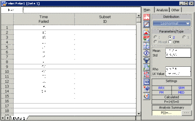
The above example can be repeated using Weibull++ , using RRY.
The mean can be obtained from the QCP and both the mean and the standard deviation can be obtained from the Function Wizard.
Rank Regression on X
Performing a rank regression on X requires that a straight line be fitted to a set of data points such that the sum of the squares of the horizontal deviations from the points to the line is minimized.
Again, the first task is to bring our [math]\displaystyle{ cdf }[/math] function into a linear form. This step is exactly the same as in regression on Y analysis and Eqns. (lnorm), (yln), (aln) and (bln) apply in this case too. The deviation from the previous analysis begins on the least squares fit part, where in this case we treat [math]\displaystyle{ x }[/math] as the dependent variable and [math]\displaystyle{ y }[/math] as the independent variable. The best-fitting straight line to the data, for regression on X (see Chapter 3), is the straight line:
- [math]\displaystyle{ x=\widehat{a}+\widehat{b}y }[/math]
The corresponding equations for and [math]\displaystyle{ \widehat{b} }[/math] are:
- [math]\displaystyle{ \hat{a}=\overline{x}-\hat{b}\overline{y}=\frac{\underset{i=1}{\overset{N}{\mathop{\sum }}}\,{{x}_{i}}}{N}-\hat{b}\frac{\underset{i=1}{\overset{N}{\mathop{\sum }}}\,{{y}_{i}}}{N} }[/math]
and:
- [math]\displaystyle{ \hat{b}=\frac{\underset{i=1}{\overset{N}{\mathop{\sum }}}\,{{x}_{i}}{{y}_{i}}-\tfrac{\underset{i=1}{\overset{N}{\mathop{\sum }}}\,{{x}_{i}}\underset{i=1}{\overset{N}{\mathop{\sum }}}\,{{y}_{i}}}{N}}{\underset{i=1}{\overset{N}{\mathop{\sum }}}\,y_{i}^{2}-\tfrac{{{\left( \underset{i=1}{\overset{N}{\mathop{\sum }}}\,{{y}_{i}} \right)}^{2}}}{N}} }[/math]
where:
- [math]\displaystyle{ {{y}_{i}}={{\Phi }^{-1}}\left[ F(T_{i}^{\prime }) \right] }[/math]
and:
- [math]\displaystyle{ {{x}_{i}}=T_{i}^{\prime } }[/math]
and the [math]\displaystyle{ F(T_{i}^{\prime }) }[/math] is estimated from the median ranks. Once [math]\displaystyle{ \widehat{a} }[/math] and [math]\displaystyle{ \widehat{b} }[/math] are obtained, solve Eqn. (xlineln) for the unknown [math]\displaystyle{ y }[/math] , which corresponds to:
- [math]\displaystyle{ y=-\frac{\widehat{a}}{\widehat{b}}+\frac{1}{\widehat{b}}x }[/math]
Solving for the parameters from Eqns. (bln) and (aln) we get:
- [math]\displaystyle{ a=-\frac{\widehat{a}}{\widehat{b}}=-\frac{{{\mu }'}}{{{\sigma }_{{{T}'}}}} }[/math]
and:
- [math]\displaystyle{ b=\frac{1}{\widehat{b}}=\frac{1}{{{\sigma }_{{{T}'}}}}\text{ } }[/math]
The correlation coefficient is evaluated as before using Eqn. (RHOln).
Example 3
Using the data of Example 2 and assuming a lognormal distribution, estimate the parameters and estimate the correlation coefficient, [math]\displaystyle{ \rho }[/math] , using rank regression on X.
Solution to Example 3
Table 9.2 constructed in Example 2 applies to this example as well. Using the values in this table we get:
- [math]\displaystyle{ \begin{align} & \hat{b}= & \frac{\underset{i=1}{\overset{14}{\mathop{\sum }}}\,T_{i}^{\prime }{{y}_{i}}-\tfrac{\underset{i=1}{\overset{14}{\mathop{\sum }}}\,T_{i}^{\prime }\underset{i=1}{\overset{14}{\mathop{\sum }}}\,{{y}_{i}}}{14}}{\underset{i=1}{\overset{14}{\mathop{\sum }}}\,y_{i}^{2}-\tfrac{{{\left( \underset{i=1}{\overset{14}{\mathop{\sum }}}\,{{y}_{i}} \right)}^{2}}}{14}} \\ & & \\ & \widehat{b}= & \frac{10.4473-(49.2220)(0)/14}{11.3646-{{(0)}^{2}}/14} \end{align} }[/math]
or:
- [math]\displaystyle{ \widehat{b}=0.9193 }[/math]
and:
- [math]\displaystyle{ \hat{a}=\overline{x}-\hat{b}\overline{y}=\frac{\underset{i=1}{\overset{14}{\mathop{\sum }}}\,T_{i}^{\prime }}{14}-\widehat{b}\frac{\underset{i=1}{\overset{14}{\mathop{\sum }}}\,{{y}_{i}}}{14} }[/math]
or:
- [math]\displaystyle{ \widehat{a}=\frac{49.2220}{14}-(0.9193)\frac{(0)}{14}=3.5159 }[/math]
Therefore, from Eqn. (blnx):
- [math]\displaystyle{ {{\sigma }_{{{T}'}}}=\widehat{b}=0.9193 }[/math]
and from Eqn. (alnx):
- [math]\displaystyle{ {\mu }'=\frac{\widehat{a}}{\widehat{b}}{{\sigma }_{{{T}'}}}=\frac{3.5159}{0.9193}\cdot 0.9193=3.5159 }[/math]
Using Eqns. (mean) and (sdv) we get:
- [math]\displaystyle{ \overline{T}=\mu =51.3393\text{ hours} }[/math]
and:
- [math]\displaystyle{ {{\sigma }_{T}}=59.1682\text{ hours}. }[/math]
The correlation coefficient is found using Eqn. (RHOln):
- [math]\displaystyle{ \widehat{\rho }=0.9754. }[/math]
Note that the regression on Y analysis is not necessarily the same as the regression on X. The only time when the results of the two regression types are the same (i.e. will yield the same equation for a line) is when the data lie perfectly on a line.
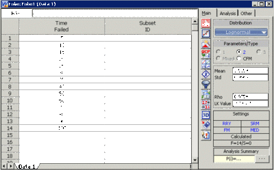
Using Weibull++ , with the Rank Regression on X option, the results are:
Maximum Likelihood Estimation
As it was outlined in Chapter 3, maximum likelihood estimation works by developing a likelihood function based on the available data and finding the values of the parameter estimates that maximize the likelihood function. This can be achieved by using iterative methods to determine the parameter estimate values that maximize the likelihood function. However, this can be rather difficult and time-consuming, particularly when dealing with the three-parameter distribution. Another method of finding the parameter estimates involves taking the partial derivatives of the likelihood equation with respect to the parameters, setting the resulting equations equal to zero, and solving simultaneously to determine the values of the parameter estimates. The log-likelihood functions and associated partial derivatives used to determine maximum likelihood estimates for the lognormal distribution are covered in Appendix C.
Confidence Bounds
The method used by the application in estimating the different types of confidence bounds for lognormally distributed data is presented in this section. Note that there are closed-form solutions for both the normal and lognormal reliability that can be obtained without the use of the Fisher information matrix. However, these closed-form solutions only apply to complete data. To achieve consistent application across all possible data types, Weibull++ always uses the Fisher matrix in computing confidence intervals. The complete derivations were presented in detail for a general function in Chapter 5. For a discussion on exact confidence bounds for the normal and lognormal, see Chapter 8.
Fisher Matrix Bounds
Bounds on the Parameters
The lower and upper bounds on the mean, [math]\displaystyle{ {\mu }' }[/math] , are estimated from:
- [math]\displaystyle{ \begin{align} & \mu _{U}^{\prime }= & {{\widehat{\mu }}^{\prime }}+{{K}_{\alpha }}\sqrt{Var({{\widehat{\mu }}^{\prime }})}\text{ (upper bound),} \\ & \mu _{L}^{\prime }= & {{\widehat{\mu }}^{\prime }}-{{K}_{\alpha }}\sqrt{Var({{\widehat{\mu }}^{\prime }})}\text{ (lower bound)}\text{.} \end{align} }[/math]
For the standard deviation, [math]\displaystyle{ {{\widehat{\sigma }}_{{{T}'}}} }[/math] , [math]\displaystyle{ \ln ({{\widehat{\sigma }}_{{{T}'}}}) }[/math] is treated as normally distributed, and the bounds are estimated from:
- [math]\displaystyle{ \begin{align} & {{\sigma }_{U}}= & {{\widehat{\sigma }}_{{{T}'}}}\cdot {{e}^{\tfrac{{{K}_{\alpha }}\sqrt{Var({{\widehat{\sigma }}_{{{T}'}}})}}{{{\widehat{\sigma }}_{{{T}'}}}}}}\text{ (upper bound),} \\ & {{\sigma }_{L}}= & \frac{{{\widehat{\sigma }}_{{{T}'}}}}{{{e}^{\tfrac{{{K}_{\alpha }}\sqrt{Var({{\widehat{\sigma }}_{{{T}'}}})}}{{{\widehat{\sigma }}_{{{T}'}}}}}}}\text{ (lower bound),} \end{align} }[/math]
where [math]\displaystyle{ {{K}_{\alpha }} }[/math] is defined by:
- [math]\displaystyle{ \alpha =\frac{1}{\sqrt{2\pi }}\int_{{{K}_{\alpha }}}^{\infty }{{e}^{-\tfrac{{{t}^{2}}}{2}}}dt=1-\Phi ({{K}_{\alpha }}) }[/math]
If [math]\displaystyle{ \delta }[/math] is the confidence level, then [math]\displaystyle{ \alpha =\tfrac{1-\delta }{2} }[/math] for the two-sided bounds and [math]\displaystyle{ \alpha =1-\delta }[/math] for the one-sided bounds.
The variances and covariances of [math]\displaystyle{ {{\widehat{\mu }}^{\prime }} }[/math] and [math]\displaystyle{ {{\widehat{\sigma }}_{{{T}'}}} }[/math] are estimated as follows:
- [math]\displaystyle{ \left( \begin{matrix} \widehat{Var}\left( {{\widehat{\mu }}^{\prime }} \right) & \widehat{Cov}\left( {{\widehat{\mu }}^{\prime }},{{\widehat{\sigma }}_{{{T}'}}} \right) \\ \widehat{Cov}\left( {{\widehat{\mu }}^{\prime }},{{\widehat{\sigma }}_{{{T}'}}} \right) & \widehat{Var}\left( {{\widehat{\sigma }}_{{{T}'}}} \right) \\ \end{matrix} \right)=\left( \begin{matrix} -\tfrac{{{\partial }^{2}}\Lambda }{\partial {{({\mu }')}^{2}}} & -\tfrac{{{\partial }^{2}}\Lambda }{\partial {\mu }'\partial {{\sigma }_{{{T}'}}}} \\ {} & {} \\ -\tfrac{{{\partial }^{2}}\Lambda }{\partial {\mu }'\partial {{\sigma }_{{{T}'}}}} & -\tfrac{{{\partial }^{2}}\Lambda }{\partial \sigma _{{{T}'}}^{2}} \\ \end{matrix} \right)_{{\mu }'={{\widehat{\mu }}^{\prime }},{{\sigma }_{{{T}'}}}={{\widehat{\sigma }}_{{{T}'}}}}^{-1} }[/math]
where [math]\displaystyle{ \Lambda }[/math] is the log-likelihood function of the lognormal distribution.
Bounds on Reliability
The reliability of the lognormal distribution is:
- [math]\displaystyle{ \hat{R}({T}';{\mu }',{{\sigma }_{{{T}'}}})=\int_{{{T}'}}^{\infty }\frac{1}{{{\widehat{\sigma }}_{{{T}'}}}\sqrt{2\pi }}{{e}^{-\tfrac{1}{2}{{\left( \tfrac{t-{{\widehat{\mu }}^{\prime }}}{{{\widehat{\sigma }}_{{{T}'}}}} \right)}^{2}}}}dt }[/math]
Let [math]\displaystyle{ \widehat{z}(t;{{\hat{\mu }}^{\prime }},{{\hat{\sigma }}_{{{T}'}}})=\tfrac{t-{{\widehat{\mu }}^{\prime }}}{{{\widehat{\sigma }}_{{{T}'}}}}, }[/math] then [math]\displaystyle{ \tfrac{d\widehat{z}}{dt}=\tfrac{1}{{{\widehat{\sigma }}_{{{T}'}}}}. }[/math] For [math]\displaystyle{ t={T}' }[/math] , [math]\displaystyle{ \widehat{z}=\tfrac{{T}'-{{\widehat{\mu }}^{\prime }}}{{{\widehat{\sigma }}_{{{T}'}}}} }[/math] , and for [math]\displaystyle{ t=\infty , }[/math] [math]\displaystyle{ \widehat{z}=\infty . }[/math] The above equation then becomes:
- [math]\displaystyle{ \hat{R}(\widehat{z})=\int_{\widehat{z}({T}')}^{\infty }\frac{1}{\sqrt{2\pi }}{{e}^{-\tfrac{1}{2}{{z}^{2}}}}dz }[/math]
The bounds on [math]\displaystyle{ z }[/math] are estimated from:
- [math]\displaystyle{ \begin{align} & {{z}_{U}}= & \widehat{z}+{{K}_{\alpha }}\sqrt{Var(\widehat{z})} \\ & {{z}_{L}}= & \widehat{z}-{{K}_{\alpha }}\sqrt{Var(\widehat{z})} \end{align} }[/math]
where:
- [math]\displaystyle{ \begin{align} & Var(\widehat{z})= & \left( \frac{\partial z}{\partial {\mu }'} \right)_{{{\widehat{\mu }}^{\prime }}}^{2}Var({{\widehat{\mu }}^{\prime }})+\left( \frac{\partial z}{\partial {{\sigma }_{{{T}'}}}} \right)_{{{\widehat{\sigma }}_{{{T}'}}}}^{2}Var({{\widehat{\sigma }}_{{{T}'}}}) \\ & & +2{{\left( \frac{\partial z}{\partial {\mu }'} \right)}_{{{\widehat{\mu }}^{\prime }}}}{{\left( \frac{\partial z}{\partial {{\sigma }_{{{T}'}}}} \right)}_{{{\widehat{\sigma }}_{{{T}'}}}}}Cov\left( {{\widehat{\mu }}^{\prime }},{{\widehat{\sigma }}_{{{T}'}}} \right) \end{align} }[/math]
or:
- [math]\displaystyle{ Var(\widehat{z})=\frac{1}{\widehat{\sigma }_{{{T}'}}^{2}}\left[ Var({{\widehat{\mu }}^{\prime }})+{{\widehat{z}}^{2}}Var({{\widehat{\sigma }}_{{{T}'}}})+2\cdot \widehat{z}\cdot Cov\left( {{\widehat{\mu }}^{\prime }},{{\widehat{\sigma }}_{{{T}'}}} \right) \right] }[/math]
The upper and lower bounds on reliability are:
- [math]\displaystyle{ \begin{align} & {{R}_{U}}= & \int_{{{z}_{L}}}^{\infty }\frac{1}{\sqrt{2\pi }}{{e}^{-\tfrac{1}{2}{{z}^{2}}}}dz\text{ (Upper bound)} \\ & {{R}_{L}}= & \int_{{{z}_{U}}}^{\infty }\frac{1}{\sqrt{2\pi }}{{e}^{-\tfrac{1}{2}{{z}^{2}}}}dz\text{ (Lower bound)} \end{align} }[/math]
Bounds on Time
The bounds around time for a given lognormal percentile, or unreliability, are estimated by first solving the reliability equation with respect to time, as follows:
- [math]\displaystyle{ {T}'({{\widehat{\mu }}^{\prime }},{{\widehat{\sigma }}_{{{T}'}}})={{\widehat{\mu }}^{\prime }}+z\cdot {{\widehat{\sigma }}_{{{T}'}}} }[/math]
where:
- [math]\displaystyle{ z={{\Phi }^{-1}}\left[ F({T}') \right] }[/math]
and:
- [math]\displaystyle{ \Phi (z)=\frac{1}{\sqrt{2\pi }}\int_{-\infty }^{z({T}')}{{e}^{-\tfrac{1}{2}{{z}^{2}}}}dz }[/math]
The next step is to calculate the variance of [math]\displaystyle{ {T}'({{\widehat{\mu }}^{\prime }},{{\widehat{\sigma }}_{{{T}'}}}): }[/math]
- [math]\displaystyle{ \begin{align} & Var({{{\hat{T}}}^{\prime }})= & {{\left( \frac{\partial {T}'}{\partial {\mu }'} \right)}^{2}}Var({{\widehat{\mu }}^{\prime }})+{{\left( \frac{\partial {T}'}{\partial {{\sigma }_{{{T}'}}}} \right)}^{2}}Var({{\widehat{\sigma }}_{{{T}'}}}) \\ & & +2\left( \frac{\partial {T}'}{\partial {\mu }'} \right)\left( \frac{\partial {T}'}{\partial {{\sigma }_{{{T}'}}}} \right)Cov\left( {{\widehat{\mu }}^{\prime }},{{\widehat{\sigma }}_{{{T}'}}} \right) \\ & & \\ & Var({{{\hat{T}}}^{\prime }})= & Var({{\widehat{\mu }}^{\prime }})+{{\widehat{z}}^{2}}Var({{\widehat{\sigma }}_{{{T}'}}})+2\cdot \widehat{z}\cdot Cov\left( {{\widehat{\mu }}^{\prime }},{{\widehat{\sigma }}_{{{T}'}}} \right) \end{align} }[/math]
The upper and lower bounds are then found by:
- [math]\displaystyle{ \begin{align} & T_{U}^{\prime }= & \ln {{T}_{U}}={{{\hat{T}}}^{\prime }}+{{K}_{\alpha }}\sqrt{Var({{{\hat{T}}}^{\prime }})} \\ & T_{L}^{\prime }= & \ln {{T}_{L}}={{{\hat{T}}}^{\prime }}-{{K}_{\alpha }}\sqrt{Var({{{\hat{T}}}^{\prime }})} \end{align} }[/math]
Solving for [math]\displaystyle{ {{T}_{U}} }[/math] and [math]\displaystyle{ {{T}_{L}} }[/math] we get:
- [math]\displaystyle{ \begin{align} & {{T}_{U}}= & {{e}^{T_{U}^{\prime }}}\text{ (upper bound),} \\ & {{T}_{L}}= & {{e}^{T_{L}^{\prime }}}\text{ (lower bound)}\text{.} \end{align} }[/math]
Example 4
Using the data of Example 2 and assuming a lognormal distribution, estimate the parameters using the MLE method.
Solution to Example 4
In this example we have only complete data. Thus, the partials reduce to:
- [math]\displaystyle{ \begin{align} & \frac{\partial \Lambda }{\partial {\mu }'}= & \frac{1}{\sigma _{{{T}'}}^{2}}\cdot \underset{i=1}{\overset{14}{\mathop \sum }}\,\ln ({{T}_{i}})-{\mu }'=0 \\ & \frac{\partial \Lambda }{\partial {{\sigma }_{{{T}'}}}}= & \underset{i=1}{\overset{14}{\mathop \sum }}\,\left( \frac{\ln ({{T}_{i}})-{\mu }'}{\sigma _{{{T}'}}^{3}}-\frac{1}{{{\sigma }_{{{T}'}}}} \right)=0 \end{align} }[/math]
Substituting the values of [math]\displaystyle{ {{T}_{i}} }[/math] and solving the above system simultaneously, we get:
- [math]\displaystyle{ \begin{align} & {{{\hat{\sigma }}}_{{{T}'}}}= & 0.849 \\ & {{{\hat{\mu }}}^{\prime }}= & 3.516 \end{align} }[/math]
Using Eqns. (mean) and (sdv) we get:
- [math]\displaystyle{ \overline{T}=\hat{\mu }=48.25\text{ hours} }[/math]
and:
- [math]\displaystyle{ {{\hat{\sigma }}_{{{T}'}}}=49.61\text{ hours}. }[/math]
The variance/covariance matrix is given by:
- [math]\displaystyle{ \left[ \begin{matrix} \widehat{Var}\left( {{{\hat{\mu }}}^{\prime }} \right)=0.0515 & {} & \widehat{Cov}\left( {{{\hat{\mu }}}^{\prime }},{{{\hat{\sigma }}}_{{{T}'}}} \right)=0.0000 \\ {} & {} & {} \\ \widehat{Cov}\left( {{{\hat{\mu }}}^{\prime }},{{{\hat{\sigma }}}_{{{T}'}}} \right)=0.0000 & {} & \widehat{Var}\left( {{{\hat{\sigma }}}_{{{T}'}}} \right)=0.0258 \\ \end{matrix} \right] }[/math]
Note About Bias
See the discussion regarding bias with the normal distribution in Chapter 8 for information regarding parameter bias in the lognormal distribution.
Likelihood Ratio Confidence Bounds
Bounds on Parameters
As covered in Chapter 5, the likelihood confidence bounds are calculated by finding values for [math]\displaystyle{ {{\theta }_{1}} }[/math] and [math]\displaystyle{ {{\theta }_{2}} }[/math] that satisfy:
- [math]\displaystyle{ -2\cdot \text{ln}\left( \frac{L({{\theta }_{1}},{{\theta }_{2}})}{L({{\widehat{\theta }}_{1}},{{\widehat{\theta }}_{2}})} \right)=\chi _{\alpha ;1}^{2} }[/math]
This equation can be rewritten as:
- [math]\displaystyle{ L({{\theta }_{1}},{{\theta }_{2}})=L({{\widehat{\theta }}_{1}},{{\widehat{\theta }}_{2}})\cdot {{e}^{\tfrac{-\chi _{\alpha ;1}^{2}}{2}}} }[/math]
For complete data, the likelihood formula for the normal distribution is given by:
- [math]\displaystyle{ L({\mu }',{{\sigma }_{{{T}'}}})=\underset{i=1}{\overset{N}{\mathop \prod }}\,f({{x}_{i}};{\mu }',{{\sigma }_{{{T}'}}})=\underset{i=1}{\overset{N}{\mathop \prod }}\,\frac{1}{{{x}_{i}}\cdot {{\sigma }_{{{T}'}}}\cdot \sqrt{2\pi }}\cdot {{e}^{-\tfrac{1}{2}{{\left( \tfrac{\text{ln}({{x}_{i}})-{\mu }'}{{{\sigma }_{{{T}'}}}} \right)}^{2}}}} }[/math]
where the [math]\displaystyle{ {{x}_{i}} }[/math] values represent the original time-to-failure data. For a given value of [math]\displaystyle{ \alpha }[/math] , values for [math]\displaystyle{ {\mu }' }[/math] and [math]\displaystyle{ {{\sigma }_{{{T}'}}} }[/math] can be found which represent the maximum and minimum values that satisfy Eqn. (lratio3). These represent the confidence bounds for the parameters at a confidence level [math]\displaystyle{ \delta , }[/math] where [math]\displaystyle{ \alpha =\delta }[/math] for two-sided bounds and [math]\displaystyle{ \alpha =2\delta -1 }[/math] for one-sided.
Example 5
Five units are put on a reliability test and experience failures at 45, 60, 75, 90, and 115 hours. Assuming a lognormal distribution, the MLE parameter estimates are calculated to be [math]\displaystyle{ {{\widehat{\mu }}^{\prime }}=4.2926 }[/math] and [math]\displaystyle{ {{\widehat{\sigma }}_{{{T}'}}}=0.32361. }[/math] Calculate the two-sided 75% confidence bounds on these parameters using the likelihood ratio method.
Solution to Example 5
The first step is to calculate the likelihood function for the parameter estimates:
where [math]\displaystyle{ {{x}_{i}} }[/math] are the original time-to-failure data points. We can now rearrange Eqn. (lratio3) to the form:
- [math]\displaystyle{ L({\mu }',{{\sigma }_{{{T}'}}})-L({{\widehat{\mu }}^{\prime }},{{\widehat{\sigma }}_{{{T}'}}})\cdot {{e}^{\tfrac{-\chi _{\alpha ;1}^{2}}{2}}}=0 }[/math]
Since our specified confidence level, [math]\displaystyle{ \delta }[/math] , is 75%, we can calculate the value of the chi-squared statistic, [math]\displaystyle{ \chi _{0.75;1}^{2}=1.323303. }[/math] We can now substitute this information into the equation:
- [math]\displaystyle{ \begin{align} & L({\mu }',{{\sigma }_{{{T}'}}})-L({{\widehat{\mu }}^{\prime }},{{\widehat{\sigma }}_{{{T}'}}})\cdot {{e}^{\tfrac{-\chi _{\alpha ;1}^{2}}{2}}}= & 0 \\ & L({\mu }',{{\sigma }_{{{T}'}}})-1.115256\times {{10}^{-10}}\cdot {{e}^{\tfrac{-1.323303}{2}}}= & 0 \\ & L({\mu }',{{\sigma }_{{{T}'}}})-5.754703\times {{10}^{-11}}= & 0 \end{align} }[/math]
It now remains to find the values of [math]\displaystyle{ {\mu }' }[/math] and [math]\displaystyle{ {{\sigma }_{{{T}'}}} }[/math] which satisfy this equation. This is an iterative process that requires setting the value of [math]\displaystyle{ {{\sigma }_{{{T}'}}} }[/math] and finding the appropriate values of [math]\displaystyle{ {\mu }' }[/math] , and vice versa.
The following table gives the values of [math]\displaystyle{ {\mu }' }[/math] based on given values of [math]\displaystyle{ {{\sigma }_{{{T}'}}} }[/math] .
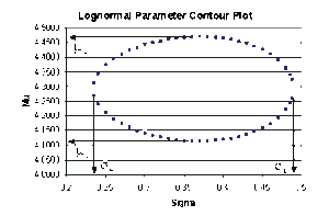
These points are represented graphically in the following contour plot:
(Note that this plot is generated with degrees of freedom [math]\displaystyle{ k=1 }[/math] , as we are only determining bounds on one parameter. The contour plots generated in Weibull++ are done with degrees of freedom [math]\displaystyle{ k=2 }[/math] , for use in comparing both parameters simultaneously.) As can be determined from the table the lowest calculated value for [math]\displaystyle{ {\mu }' }[/math] is 4.1145, while the highest is 4.4708. These represent the two-sided 75% confidence limits on this parameter. Since solutions for the equation do not exist for values of [math]\displaystyle{ {{\sigma }_{{{T}'}}} }[/math] below 0.24 or above 0.48, these can be considered the two-sided 75% confidence limits for this parameter. In order to obtain more accurate values for the confidence limits on [math]\displaystyle{ {{\sigma }_{{{T}'}}} }[/math] , we can perform the same procedure as before, but finding the two values of [math]\displaystyle{ \sigma }[/math] that correspond with a given value of [math]\displaystyle{ {\mu }'. }[/math] Using this method, we find that the 75% confidence limits on [math]\displaystyle{ {{\sigma }_{{{T}'}}} }[/math] are 0.23405 and 0.48936, which are close to the initial estimates of 0.24 and 0.48.
Bounds on Time and Reliability
In order to calculate the bounds on a time estimate for a given reliability, or on a reliability estimate for a given time, the likelihood function needs to be rewritten in terms of one parameter and time/reliability, so that the maximum and minimum values of the time can be observed as the parameter is varied. This can be accomplished by substituting a form of the normal reliability equation into the likelihood function. The normal reliability equation can be written as:
- [math]\displaystyle{ R=1-\Phi \left( \frac{\text{ln}(t)-{\mu }'}{{{\sigma }_{{{T}'}}}} \right) }[/math]
This can be rearranged to the form:
- [math]\displaystyle{ {\mu }'=\text{ln}(t)-{{\sigma }_{{{T}'}}}\cdot {{\Phi }^{-1}}(1-R) }[/math]
where [math]\displaystyle{ {{\Phi }^{-1}} }[/math] is the inverse standard normal. This equation can now be substituted into Eqn. (lognormlikelihood) to produce a likelihood equation in terms of [math]\displaystyle{ {{\sigma }_{{{T}'}}}, }[/math] [math]\displaystyle{ t }[/math] and [math]\displaystyle{ R\ \ : }[/math]
- [math]\displaystyle{ L({{\sigma }_{{{T}'}}},t/R)=\underset{i=1}{\overset{N}{\mathop \prod }}\,\frac{1}{{{x}_{i}}\cdot {{\sigma }_{{{T}'}}}\cdot \sqrt{2\pi }}\cdot {{e}^{-\tfrac{1}{2}{{\left( \tfrac{\text{ln}({{x}_{i}})-\left( \text{ln}(t)-{{\sigma }_{{{T}'}}}\cdot {{\Phi }^{-1}}(1-R) \right)}{{{\sigma }_{{{T}'}}}} \right)}^{2}}}} }[/math]
The unknown variable [math]\displaystyle{ t/R }[/math] depends on what type of bounds are being determined. If one is trying to determine the bounds on time for a given reliability, then [math]\displaystyle{ R }[/math] is a known constant and [math]\displaystyle{ t }[/math] is the unknown variable. Conversely, if one is trying to determine the bounds on reliability for a given time, then [math]\displaystyle{ t }[/math] is a known constant and [math]\displaystyle{ R }[/math] is the unknown variable. Either way, Eqn. (lognormliketr) can be used to solve Eqn. (lratio3) for the values of interest.
Example 6
For the data given in Example 5, determine the two-sided 75% confidence bounds on the time estimate for a reliability of 80%. The ML estimate for the time at [math]\displaystyle{ R(t)=80% }[/math] is 55.718.
Solution to Example 6
In this example, we are trying to determine the two-sided 75% confidence bounds on the time estimate of 55.718. This is accomplished by substituting [math]\displaystyle{ R=0.80 }[/math] and [math]\displaystyle{ \alpha =0.75 }[/math] into Eqn. (lognormliketr), and varying [math]\displaystyle{ {{\sigma }_{{{T}'}}} }[/math] until the maximum and minimum values of [math]\displaystyle{ t }[/math] are found. The following table gives the values of [math]\displaystyle{ t }[/math] based on given values of [math]\displaystyle{ {{\sigma }_{{{T}'}}} }[/math] .
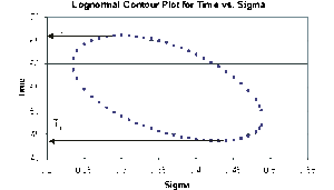
This data set is represented graphically in the following contour plot:
As can be determined from the table, the lowest calculated value for [math]\displaystyle{ t }[/math] is 43.634, while the highest is 66.085. These represent the two-sided 75% confidence limits on the time at which reliability is equal to 80%.
Example 7
For the data given in Example 5, determine the two-sided 75% confidence bounds on the reliability estimate for [math]\displaystyle{ t=65 }[/math] . The ML estimate for the reliability at [math]\displaystyle{ t=65 }[/math] is 64.261%.
Solution to Example 7
In this example, we are trying to determine the two-sided 75% confidence bounds on the reliability estimate of 64.261%. This is accomplished by substituting [math]\displaystyle{ t=65 }[/math] and [math]\displaystyle{ \alpha =0.75 }[/math] into Eqn. (lognormliketr), and varying [math]\displaystyle{ {{\sigma }_{{{T}'}}} }[/math] until the maximum and minimum values of [math]\displaystyle{ R }[/math] are found. The following table gives the values of [math]\displaystyle{ R }[/math] based on given values of [math]\displaystyle{ {{\sigma }_{{{T}'}}} }[/math] .
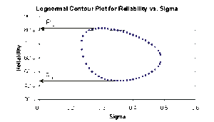
This data set is represented graphically in the following contour plot:
As can be determined from the table, the lowest calculated value for [math]\displaystyle{ R }[/math] is 43.444%, while the highest is 81.508%. These represent the two-sided 75% confidence limits on the reliability at [math]\displaystyle{ t=65 }[/math] .
Bayesian Confidence Bounds
Bounds on Parameters
From Chapter 5, we know that the marginal distribution of parameter [math]\displaystyle{ {\mu }' }[/math] is:
- [math]\displaystyle{ \begin{align} f({\mu }'|Data)= & \int_{0}^{\infty }f({\mu }',{{\sigma }_{{{T}'}}}|Data)d{{\sigma }_{{{T}'}}} \\ = & \frac{\int_{0}^{\infty }L(Data|{\mu }',{{\sigma }_{{{T}'}}})\varphi ({\mu }')\varphi ({{\sigma }_{{{T}'}}})d{{\sigma }_{{{T}'}}}}{\int_{0}^{\infty }\int_{-\infty }^{\infty }L(Data|{\mu }',{{\sigma }_{{{T}'}}})\varphi ({\mu }')\varphi ({{\sigma }_{{{T}'}}})d{\mu }'d{{\sigma }_{{{T}'}}}} \end{align} }[/math]
where:
- [math]\displaystyle{ \varphi ({{\sigma }_{{{T}'}}}) }[/math] is [math]\displaystyle{ \tfrac{1}{{{\sigma }_{{{T}'}}}} }[/math] , non-informative prior of [math]\displaystyle{ {{\sigma }_{{{T}'}}} }[/math] .
[math]\displaystyle{ \varphi ({\mu }') }[/math] is an uniform distribution from - [math]\displaystyle{ \infty }[/math] to + [math]\displaystyle{ \infty }[/math] , non-informative prior of [math]\displaystyle{ {\mu }' }[/math] . With the above prior distributions, [math]\displaystyle{ f({\mu }'|Data) }[/math] can be rewritten as:
- [math]\displaystyle{ f({\mu }'|Data)=\frac{\int_{0}^{\infty }L(Data|{\mu }',{{\sigma }_{{{T}'}}})\tfrac{1}{{{\sigma }_{{{T}'}}}}d{{\sigma }_{{{T}'}}}}{\int_{0}^{\infty }\int_{-\infty }^{\infty }L(Data|{\mu }',{{\sigma }_{{{T}'}}})\tfrac{1}{{{\sigma }_{{{T}'}}}}d{\mu }'d{{\sigma }_{{{T}'}}}} }[/math]
The one-sided upper bound of [math]\displaystyle{ {\mu }' }[/math] is:
- [math]\displaystyle{ CL=P({\mu }'\le \mu _{U}^{\prime })=\int_{-\infty }^{\mu _{U}^{\prime }}f({\mu }'|Data)d{\mu }' }[/math]
The one-sided lower bound of [math]\displaystyle{ {\mu }' }[/math] is:
- [math]\displaystyle{ 1-CL=P({\mu }'\le \mu _{L}^{\prime })=\int_{-\infty }^{\mu _{L}^{\prime }}f({\mu }'|Data)d{\mu }' }[/math]
The two-sided bounds of [math]\displaystyle{ {\mu }' }[/math] is:
- [math]\displaystyle{ CL=P(\mu _{L}^{\prime }\le {\mu }'\le \mu _{U}^{\prime })=\int_{\mu _{L}^{\prime }}^{\mu _{U}^{\prime }}f({\mu }'|Data)d{\mu }' }[/math]
The same method can be used to obtained the bounds of [math]\displaystyle{ {{\sigma }_{{{T}'}}} }[/math] .
Bounds on Time (Type 1)
The reliable life of the lognormal distribution is:
- [math]\displaystyle{ \ln T={\mu }'+{{\sigma }_{{{T}'}}}{{\Phi }^{-1}}(1-R) }[/math]
The one-sided upper on time bound is given by:
- [math]\displaystyle{ CL=\underset{}{\overset{}{\mathop{\Pr }}}\,(\ln T\le \ln {{T}_{U}})=\underset{}{\overset{}{\mathop{\Pr }}}\,({\mu }'+{{\sigma }_{{{T}'}}}{{\Phi }^{-1}}(1-R)\le \ln {{T}_{U}}) }[/math]
Eqn. (1SBT) can be rewritten in terms of [math]\displaystyle{ {\mu }' }[/math] as:
- [math]\displaystyle{ CL=\underset{}{\overset{}{\mathop{\Pr }}}\,({\mu }'\le \ln {{T}_{U}}-{{\sigma }_{{{T}'}}}{{\Phi }^{-1}}(1-R) }[/math]
From the posterior distribution of [math]\displaystyle{ {\mu }' }[/math] get:
- [math]\displaystyle{ CL=\frac{\int_{0}^{\infty }\int_{-\infty }^{\ln {{T}_{U}}-{{\sigma }_{{{T}'}}}{{\Phi }^{-1}}(1-R)}L({{\sigma }_{{{T}'}}},{\mu }')\tfrac{1}{{{\sigma }_{{{T}'}}}}d{\mu }'d{{\sigma }_{{{T}'}}}}{\int_{0}^{\infty }\int_{-\infty }^{\infty }L({{\sigma }_{{{T}'}}},{\mu }')\tfrac{1}{{{\sigma }_{{{T}'}}}}d{\mu }'d{{\sigma }_{{{T}'}}}} }[/math]
Eqn. (1SCBT) is solved w.r.t. [math]\displaystyle{ {{T}_{U}}. }[/math] The same method can be applied for one-sided lower bounds and two-sided bounds on Time.
Bounds on Reliability (Type 2)
The one-sided upper bound on reliability is given by:
- [math]\displaystyle{ CL=\underset{}{\overset{}{\mathop{\Pr }}}\,(R\le {{R}_{U}})=\underset{}{\overset{}{\mathop{\Pr }}}\,({\mu }'\le \ln T-{{\sigma }_{{{T}'}}}{{\Phi }^{-1}}(1-{{R}_{U}})) }[/math]
From the posterior distribution of [math]\displaystyle{ {\mu }' }[/math] is:
- [math]\displaystyle{ CL=\frac{\int_{0}^{\infty }\int_{-\infty }^{\ln T-{{\sigma }_{{{T}'}}}{{\Phi }^{-1}}(1-{{R}_{U}})}L({{\sigma }_{{{T}'}}},{\mu }')\tfrac{1}{{{\sigma }_{{{T}'}}}}d{\mu }'d{{\sigma }_{{{T}'}}}}{\int_{0}^{\infty }\int_{-\infty }^{\infty }L({{\sigma }_{{{T}'}}},{\mu }')\tfrac{1}{{{\sigma }_{{{T}'}}}}d{\mu }'d{{\sigma }_{{{T}'}}}} }[/math]
Eqn. (1SCBR) is solved w.r.t. [math]\displaystyle{ {{R}_{U}}. }[/math] The same method is used to calculate the one-sided lower bounds and two-sided bounds on Reliability.
Example 8
Determine the two-sided 90% Bayesian confidence bounds on the lognormal parameter estimates for the data given next:
Solution to Example 8
The data is entered into a Times-to-failure data sheet. The lognormal distribution is selected under Distributions. The Bayesian confidence bounds method only applies for the MLE analysis method, therefore, Maximum Likelihood (MLE) is selected under Analysis Method and Use Bayesian is selected under the Confidence Bounds Method in the Analysis tab.
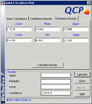
The two-sided 90% Bayesian confidence bounds on the lognormal parameter are obtained using the QCP and clicking on the Calculate Bounds button in the Parameter Bounds tab as follows:
[math]\displaystyle{ }[/math]
General Examples
Example 9
Determine the lognormal parameter estimates for the data given in Table 9.3.
| Table 9.3 - Non-Grouped Data Times-to-Failure with intervals (lnterval and left censored) | ||
| Data point index | Last Inspected | State End Time |
| 1 | 30 | 32 |
| 2 | 32 | 35 |
| 3 | 35 | 37 |
| 4 | 37 | 40 |
| 5 | 42 | 42 |
| 6 | 45 | 45 |
| 7 | 50 | 50 |
| 8 | 55 | 55 |
Solution to Example 9
This is a sequence of interval times-to-failure where the intervals vary substantially in length. Using Weibull++, the computed parameters for maximum likelihood are calculated to be:
- [math]\displaystyle{ \begin{align} & {{{\hat{\mu }}}^{\prime }}= & 3.64 \\ & {{{\hat{\sigma }}}_{{{T}'}}}= & 0.18 \end{align} }[/math]
For rank regression on [math]\displaystyle{ X\ \ : }[/math]
- [math]\displaystyle{ \begin{align} & {{{\hat{\mu }}}^{\prime }}= & 3.64 \\ & {{{\hat{\sigma }}}_{{{T}'}}}= & 0.17 \end{align} }[/math]
For rank regression on [math]\displaystyle{ Y\ \ : }[/math]
- [math]\displaystyle{ \begin{align} & {{{\hat{\mu }}}^{\prime }}= & 3.64 \\ & {{{\hat{\sigma }}}_{{{T}'}}}= & 0.21 \end{align} }[/math]
Example 10
Determine the lognormal parameter estimates for the data given in Table 9.4.
| Table 9.4 - Non-Grouped Data for Example 12 | ||
| Data point index | State F or S | State End Time |
| 1 | F | 2 |
| 2 | F | 5 |
| 3 | F | 11 |
| 4 | F | 23 |
| 5 | F | 29 |
| 6 | F | 37 |
| 7 | F | 43 |
| 8 | F | 59 |
Solution to Example 10
Using Weibull++, the computed parameters for maximum likelihood are:
- [math]\displaystyle{ \begin{align} & {{{\hat{\mu }}}^{\prime }}= & 2.83 \\ & {{{\hat{\sigma }}}_{{{T}'}}}= & 1.10 \end{align} }[/math]
For rank regression on [math]\displaystyle{ X\ \ : }[/math]
- [math]\displaystyle{ \begin{align} & {{{\hat{\mu }}}^{\prime }}= & 2.83 \\ & {{{\hat{\sigma }}}_{{{T}'}}}= & 1.24 \end{align} }[/math]
For rank regression on [math]\displaystyle{ Y\ \ : }[/math]
- [math]\displaystyle{ \begin{align} & {{{\hat{\mu }}}^{\prime }}= & 2.83 \\ & {{{\hat{\sigma }}}_{{{T}'}}}= & 1.36 \end{align} }[/math]
Example 11
From Kececioglu [19, p. 406]. Nine identical units are tested continuously to failure and their times-to-failure were recorded at 30.4, 36.7, 53.3, 58.5, 74.0, 99.3, 114.3, 140.1, and 257.9 hours.
Solution to Example 11
The results published were obtained by using the unbiased model. Published Results (using MLE):
- [math]\displaystyle{ \begin{matrix} {{\widehat{\mu }}^{\prime }}=4.3553 \\ {{\widehat{\sigma }}_{{{T}'}}}=0.67677 \\ \end{matrix} }[/math]
This same data set can be entered into Weibull++ by creating a data sheet capable of handling non-grouped time-to-failure data. Since the results shown above are unbiased, the Use Unbiased Std on Normal Data option in the User Setup must be selected in order to duplicate these results.
Weibull++ computed parameters for maximum likelihood are:
- [math]\displaystyle{ \begin{matrix} {{\widehat{\mu }}^{\prime }}=4.3553 \\ {{\widehat{\sigma }}_{{{T}'}}}=0.6768 \\ \end{matrix} }[/math]
Example 12
From Kececioglu [20, p. 347]. Fifteen identical units were tested to failure and following is a table of their times-to-failure:
Solution to Example 12
Published results (using probability plotting):
- [math]\displaystyle{ \begin{matrix} {{\widehat{\mu }}^{\prime }}=5.22575 \\ {{\widehat{\sigma }}_{{{T}'}}}=0.62048. \\ \end{matrix} }[/math]
Weibull++ computed parameters for rank regression on X are:
- [math]\displaystyle{ \begin{matrix} {{\widehat{\mu }}^{\prime }}=5.2303 \\ {{\widehat{\sigma }}_{{{T}'}}}=0.6283. \\ \end{matrix} }[/math]
The small differences are due to the precision errors when fitting a line manually, whereas in Weibull++ the line was fitted mathematically.
Example 13
From Nelson [30, p. 324]. Ninety-six locomotive controls were tested, 37 failed and 59 were suspended after running for 135,000 miles. Table 9.6 (at the end of this chapter) shows their times-to-failure.
Solution to Example 13
The distribution used in the publication was the base-10 lognormal. Published results (using MLE):
- [math]\displaystyle{ \begin{matrix} {{\widehat{\mu }}^{\prime }}=2.2223 \\ {{\widehat{\sigma }}_{{{T}'}}}=0.3064 \\ \end{matrix} }[/math]
Published 95% confidence limits on the parameters:
- [math]\displaystyle{ \begin{matrix} {{\widehat{\mu }}^{\prime }}=\left\{ 2.1336,2.3109 \right\} \\ {{\widehat{\sigma }}_{{{T}'}}}=\left\{ 0.2365,0.3970 \right\} \\ \end{matrix} }[/math]
Published variance/covariance matrix:
- [math]\displaystyle{ \left[ \begin{matrix} \widehat{Var}\left( {{{\hat{\mu }}}^{\prime }} \right)=0.0020 & {} & \widehat{Cov}({{{\hat{\mu }}}^{\prime }},{{{\hat{\sigma }}}_{{{T}'}}})=0.001 \\ {} & {} & {} \\ \widehat{Cov}({{{\hat{\mu }}}^{\prime }},{{{\hat{\sigma }}}_{{{T}'}}})=0.001 & {} & \widehat{Var}\left( {{{\hat{\sigma }}}_{{{T}'}}} \right)=0.0016 \\ \end{matrix} \right] }[/math]
To replicate the published results (since Weibull++ uses a lognormal to the base [math]\displaystyle{ e }[/math] ), take the base-10 logarithm of the data and estimate the parameters using the Normal distribution and MLE.
• Weibull++ computed parameters for maximum likelihood are:
- [math]\displaystyle{ \begin{matrix} {{\widehat{\mu }}^{\prime }}=2.2223 \\ {{\widehat{\sigma }}_{{{T}'}}}=0.3064 \\ \end{matrix} }[/math]
• Weibull++ computed 95% confidence limits on the parameters:
- [math]\displaystyle{ \begin{matrix} {{\widehat{\mu }}^{\prime }}=\left\{ 2.1364,2.3081 \right\} \\ {{\widehat{\sigma }}_{{{T}'}}}=\left\{ 0.2395,0.3920 \right\} \\ \end{matrix} }[/math]
• Weibull++ computed/variance covariance matrix:
- [math]\displaystyle{ \left[ \begin{matrix} \widehat{Var}\left( {{{\hat{\mu }}}^{\prime }} \right)=0.0019 & {} & \widehat{Cov}({{{\hat{\mu }}}^{\prime }},{{{\hat{\sigma }}}_{{{T}'}}})=0.0009 \\ {} & {} & {} \\ \widehat{Cov}({\mu }',{{{\hat{\sigma }}}_{{{T}'}}})=0.0009 & {} & \widehat{Var}\left( {{{\hat{\sigma }}}_{{{T}'}}} \right)=0.0015 \\ \end{matrix} \right] }[/math]
| Table 9.6 - Nelson's Locomotive Data | |||
| Number in State | F or S | Time | |
|---|---|---|---|
| 1 | 1 | F | 22.5 |
| 2 | 1 | F | 37.5 |
| 3 | 1 | F | 46 |
| 4 | 1 | F | 48.5 |
| 5 | 1 | F | 51.5 |
| 6 | 1 | F | 53 |
| 7 | 1 | F | 54.5 |
| 8 | 1 | F | 57.5 |
| 9 | 1 | F | 66.5 |
| 10 | 1 | F | 68 |
| 11 | 1 | F | 69.5 |
| 12 | 1 | F | 76.5 |
| 13 | 1 | F | 77 |
| 14 | 1 | F | 78.5 |
| 15 | 1 | F | 80 |
| 16 | 1 | F | 81.5 |
| 17 | 1 | F | 82 |
| 18 | 1 | F | 83 |
| 19 | 1 | F | 84 |
| 20 | 1 | F | 91.5 |
| 21 | 1 | F | 93.5 |
| 22 | 1 | F | 102.5 |
| 23 | 1 | F | 107 |
| 24 | 1 | F | 108.5 |
| 25 | 1 | F | 112.5 |
| 26 | 1 | F | 113.5 |
| 27 | 1 | F | 116 |
| 28 | 1 | F | 117 |
| 29 | 1 | F | 118.5 |
| 30 | 1 | F | 119 |
| 31 | 1 | F | 120 |
| 32 | 1 | F | 122.5 |
| 33 | 1 | F | 123 |
| 34 | 1 | F | 127.5 |
| 35 | 1 | F | 131 |
| 36 | 1 | F | 132.5 |
| 37 | 1 | F | 134 |
| 38 | 59 | S | 135 |

