Degradation Data Analysis

Given that products are more frequently being designed with higher reliability and developed in a shorter amount of time, it is often not possible to test new designs to failure under normal operating conditions. In some cases, it is possible to infer the reliability behavior of unfailed test samples with only the accumulated test time information and assumptions about the distribution. However, this generally leads to a great deal of uncertainty in the results. Another option in this situation is the use of degradation analysis. Degradation analysis involves the measurement of performance data that can be directly related to the presumed failure of the product in question. Many failure mechanisms can be directly linked to the degradation of part of the product, and degradation analysis allows the analyst to extrapolate to an assumed failure time based on the measurements of degradation over time.

In some cases, it is possible to directly measure the degradation of a physical characteristic over time, as with the wear of brake pads, the propagation of crack size, or the degradation of a performance characteristic over time such as the voltage of a battery or the luminous flux of an LED bulb. These cases belong to the Non-Destructive Degradation Analysis category. In other cases, direct measurement of degradation might not be possible without invasive or destructive measurement techniques that would directly affect the subsequent performance of the product; therefore, only one degradation measurement is possible. Examples are the measurement of corrosion in a chemical container or the strength measurement of an adhesive bond. These cases belong to the Destructive Degradation Analysis Category. In either case, however, it is necessary to be able to define a level of degradation or performance at which a failure is said to have occurred.

With this failure level defined, it is a relatively simple matter to use basic mathematical models to extrapolate the measurements over time to the point where the failure is said to occur. Once these have been determined, it is merely a matter of analyzing the extrapolated failure times in the same manner as conventional time-to-failure data.

Non-Destructive Degradation Analysis

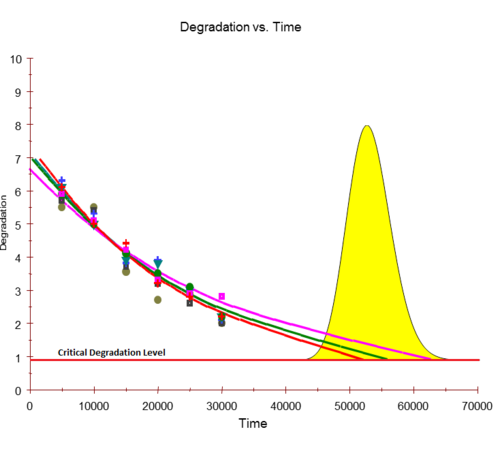
The Non-Destructive Degradation Analysis applies to cases where multiple degradation measurements over time can be obtained for each sample in the test. Given a defined level of failure (or the degradation level that would constitute a failure), basic mathematical models are used to extrapolate the degradation measurements over time of each sample to the point in time where the failure will occur. Once these extrapolated failure times are obtained, it is merely a matter of analyzing the extrapolated failure times in the same manner as conventional time-to-failure data. As with conventional life data analysis, the amount of certainty in the results is directly related to the number of samples being tested. The following figure combines the steps of the analysis by showing the extrapolation of the degradation measurements to a failure time and the subsequent distribution analysis of these failure times.

Non-Destructive Degradation Models

Once the degradation information has been recorded, the next task is to extrapolate the measurements to the defined failure level in order to estimate the failure time. Weibull++ allows the user to perform such extrapolation using a linear, exponential, power or logarithmic model. These models have the following forms:

• Linear: [math]\displaystyle{ y=a\cdot x+b \! }[/math]
• Exponential: [math]\displaystyle{ y=b\cdot {{e}^{a\cdot x}}\! }[/math]
• Power: [math]\displaystyle{ y=b\cdot {{x}^{a}} \! }[/math]
• Logarithmic: [math]\displaystyle{ y=a\cdot ln(x)+b \! }[/math]
• Gompertz: [math]\displaystyle{ y=a\cdot {{b}^{{{c}^{x}}}} \! }[/math]
• Lloyd-Lipow: [math]\displaystyle{ y=a-\frac{b}{x} \! }[/math]

where [math]\displaystyle{ y\,\! }[/math] represents the performance, [math]\displaystyle{ x\,\! }[/math] represents time, and [math]\displaystyle{ a,\,\! }[/math] [math]\displaystyle{ b\,\! }[/math] and [math]\displaystyle{ c\,\! }[/math] are model parameters to be solved for.

Once the model parameters [math]\displaystyle{ {{a}_{i}}\,\! }[/math], [math]\displaystyle{ {{b}_{i}}\,\! }[/math] and [math]\displaystyle{ {{c}_{i}}\,\! }[/math] are estimated for each sample [math]\displaystyle{ i\,\! }[/math], a time [math]\displaystyle{ {{x}_{i}}\,\! }[/math] can be extrapolated, which corresponds to the defined level of failure [math]\displaystyle{ y\,\! }[/math]. The computed [math]\displaystyle{ {{x}_{i}}\,\! }[/math] values can now be used as our times-to-failure for subsequent life data analysis. As with any sort of extrapolation, one must be careful not to extrapolate too far beyond the actual range of data in order to avoid large inaccuracies (modeling errors).

Example

Crack Propagation Example (Point Estimation)

Five turbine blades are tested for crack propagation. The test units are cyclically stressed and inspected every 100,000 cycles for crack length. Failure is defined as a crack of length 30mm or greater. The following table shows the test results for the five units at each cycle:

[math]\displaystyle{ \begin{matrix} Cycles (x1000) & Unit A (mm)& Unit B (mm) & Unit C (mm) & Unit D (mm)& Unit E (mm) \\ 100 & 15 & 10 & 17 & 12 & 10 \\ 200 & 20& 15 & 25 & 16 & 15 \\ 300 & 22 & 20 &26 & 17 & 20 \\ 400 & 26 &25 & 27 & 20 & 26 \\ 500 & 29 & 30 & 33 &26 & 33 \\ \end{matrix}\,\! }[/math]

Use the exponential degradation model to extrapolate the times-to-failure data.

Solution

The first step is to solve the equation [math]\displaystyle{ y=b\cdot {{e}^{a\cdot x}}\,\! }[/math] for [math]\displaystyle{ a\,\! }[/math] and [math]\displaystyle{ b\,\! }[/math] for each of the test units. Using regression analysis, the values for each of the test units are:

[math]\displaystyle{ \begin{matrix} {} & a & b \\ Unit A & 0.00158 & 13.596 \\ Unit B & 0.00271 & 8.272 \\ Unit C & 0.00140 & 16.435 \\ Unit D & 0.00177 & 10.361 \\ Unit E & 0.00294 & 7.931 \\ \end{matrix}\,\! }[/math]

Substituting the values into the underlying exponential model, solve for [math]\displaystyle{ x\,\! }[/math] or:

[math]\displaystyle{ x=\frac{\text{ln}(y)-\text{ln}(b)}{a}\,\! }[/math]

Using the values of [math]\displaystyle{ a\,\! }[/math] and [math]\displaystyle{ b\,\! }[/math], with [math]\displaystyle{ y=30\,\! }[/math], the resulting time at which the crack length reaches 30mm can then found for each sample:

[math]\displaystyle{ \begin{matrix} {} & Cycles-to-Failure \\ Unit A & \text{500,622} \\ Unit B & \text{475,739} \\ Unit C & \text{428,739} \\ Unit D & \text{600,810} \\ Unit E & \text{452,832} \\ \end{matrix}\,\! }[/math]

These times-to-failure can now be analyzed using traditional life data analysis to obtain metrics such as the probability of failure, B10 life, mean life, etc. This analysis can be automatically performed in the Weibull++ degradation analysis folio.

Using Extrapolated Intervals

The parameters in a degradation model are estimated using available degradation data. If the data is large, the uncertainty of the estimated parameters will be small; otherwise, the uncertainty will be large. Since the failure time for a test unit is predicted based on the estimated model, we sometimes would like to see how the parameter uncertainty affects the failure time prediction. Let’s use the exponential model as an example. Assume that the critical degradation value is [math]\displaystyle{ {{y}_{crit}}\,\! }[/math]. The predicted failure time will be

[math]\displaystyle{ \hat{x}=\frac{\ln ({{y}_{crit}})-\ln (\hat{b})}{{\hat{a}}}\,\! }[/math]

The variance of the predicted failure time will be:

[math]\displaystyle{ Var(\hat{x})={{\left( \frac{\partial x}{\partial a} \right)}^{2}}Var(\hat{a})+{{\left( \frac{\partial x}{\partial b} \right)}^{2}}Var(\hat{b})+2\left( \frac{\partial x}{\partial a} \right)\left( \frac{\partial x}{\partial b} \right)Cov(\hat{a},\hat{b})\,\! }[/math]

The variance and covariance of the model parameters are calculated from using Least Squares Estimation. The details of the calculation are not given here.

The 2-sided upper and lower bounds for the predicted failure time, with a confidence level of [math]\displaystyle{ 1-\alpha \,\! }[/math] are:

[math]\displaystyle{ {{x}_{U}}=\hat{x}+{{K}_{1-\alpha /2}}\sqrt{Var(\hat{x})}\,\! }[/math]

[math]\displaystyle{ {{x}_{L}}=\hat{x}-{{K}_{1-\alpha /2}}\sqrt{Var(\hat{x})}\,\! }[/math]

In Weibull++, the confidence level used is 90%.

Example

Crack Propagation Example (Extrapolated Intervals)

Using the same data set from the previous example, predict the interval failure times for the turbine blades.

Solution

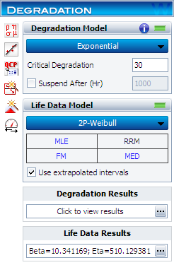
In the Weibull++ degradation analysis folio, select the Use extrapolated intervals check box, as shown next.

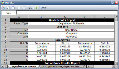
Use the exponential degradation model for the degradation analysis, and the Weibull distribution parameters with MLE for the life data analysis. The following report shows the estimated degradation model parameters.

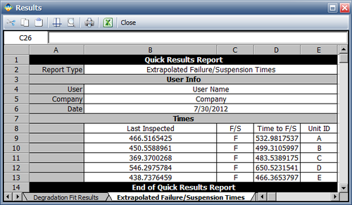
The following report shows the extrapolated failure time intervals.

Destructive Degradation Analysis

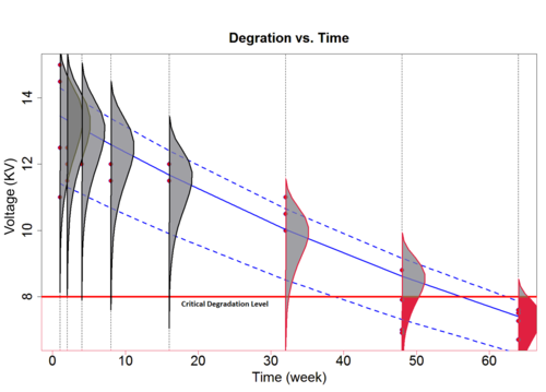
The Destructive Degradation Analysis applies to cases where the sample has to be destroyed in order to obtain a degradation measurement. As a result, degradation measurements for multiple samples are required at different points in time. The analysis performed is very similar to Accelerated Life Testing Analysis (ALTA). In this case, the "stress" used in ALTA becomes time, while the random variable becomes the degradation measurement instead of the time-to-failure. Given a defined level of failure (or the degradation level that would constitute a failure), the probability that the degradation measurement will be beyond that level at a given time can be obtained. The following plot shows the relationship between the distribution of the degradation measurement and time. The red shaded area of the last two pdfs represents the probability that the degradation measurement will be less than the critical degradation level at the corresponding times.

Destructive Degradation Models

The first step of destructive degradation analysis involves using a statistical distribution to represent the variability of a degradation measurement at a given time. The following distributions can be used:

• Weibull
• Exponential
• Normal
• Lognormal
• Gumbel

Similar to accelerated life testing analysis, the assumption is that the location or log-location parameter of the degradation measurement distribution will change with time while the shape parameter will remain constant. For each distribution:

• Weibull: [math]\displaystyle{ \ln (\eta )\,\! }[/math] is set as a function of time while [math]\displaystyle{ \beta \,\! }[/math] remains constant.
• Exponential: [math]\displaystyle{ \ln (MTTF)\,\! }[/math] is set as a function of time.
• Normal: [math]\displaystyle{ \mu \,\! }[/math] is set as a function of time while [math]\displaystyle{ \sigma \,\! }[/math] remains constant.
• Lognormal: [math]\displaystyle{ {\mu }'\,\! }[/math] is set as a function of time while [math]\displaystyle{ {\sigma }'\,\! }[/math] remains constant.
• Gumbel: [math]\displaystyle{ \mu \,\! }[/math] is set as a function of time while [math]\displaystyle{ \sigma \,\! }[/math] remains constant.

Finally, given the selected distribution, a degradation model is used to represent the change of the location (or log-location) parameter with time. The following degradation models can be used:

• Linear: [math]\displaystyle{ \mu (t)=b+a\times t \,\! }[/math]
• Exponential: [math]\displaystyle{ \mu (t)=b\times {{e}^{a\times t}}\,\! }[/math]
• Power: [math]\displaystyle{ \mu (t)=b\times {{t}^{a}}\,\! }[/math]
• Logarithm: [math]\displaystyle{ \mu (t)=a\times \ln (t)+b\,\! }[/math]
• Lloyd-Lipow: [math]\displaystyle{ \mu (t)=a-\frac{b}{t}\,\! }[/math]

The distribution and degradation models parameters are then calculated using Maximum Likelihood Estimation (MLE).

For example, if a normal distribution is used to represent the degradation measurement and a linear degradation model is assumed, then the standard deviation, [math]\displaystyle{ \sigma \,\! }[/math], will be assumed constant with time, and the mean, [math]\displaystyle{ \mu \,\! }[/math], will be:

[math]\displaystyle{ \mu (t)=b+a\times t\,\! }[/math]

The CDF of the degradation measurement [math]\displaystyle{ x(t)\,\! }[/math] is:

[math]\displaystyle{ \Pr (x(t)\lt X)=\Phi \left( \frac{X-\mu (t)}{\sigma } \right)\,\! }[/math]

Given the CDF, the parameters [math]\displaystyle{ \sigma \,\! }[/math], [math]\displaystyle{ b\,\! }[/math] and [math]\displaystyle{ a\,\! }[/math] are estimated using Maximum Likelihood Estimation.

Assuming that the requirement is that the measurement needs to be greater than a critical degradation value [math]\displaystyle{ {{D}_{crit}}\,\! }[/math] for the product to fail, the probability of failure at time [math]\displaystyle{ t\,\! }[/math] will be:

[math]\displaystyle{ F(t)=\Pr (x(t)\gt {{D}_{crit}})=1-\Phi \left( \frac{{{D}_{crit}}-\mu (t)}{\sigma } \right)\,\! }[/math]

It should be noted that the failure threshold could be specified as a degradation measurement less than (for the case of decreasing degradation) or greater than (for the case of increasing degradation) a critical degradation value.

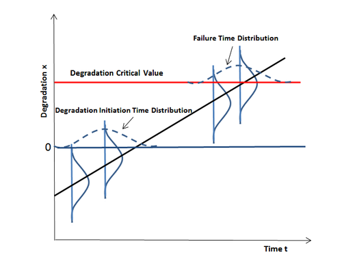
The relationship between the distribution of degradation measurement and the distribution of failure time is illustrated in the following plot.

Example

A company has been collecting degradation data over a period of 4 years with the purpose of calculating reliability after 5 years. With the degradation measurement decreasing with time, failure is defined as a measurement of 150 or below. In order to obtain such measurements, the unit has to be destroyed and therefore removed from the population.

The following table gives the degradation measurements over 4 years.

[math]\displaystyle{ \begin{matrix} Year 1 & Year 2 & Year 3 & Year 4 & \\ 437 & 412 & 246 & 125 \\ 446 & 420 & 324 & 208 \\ 497 & 451 & 330 & 229 \\ 503 & 454 & 426 & 242 \\ 705 & 554 & 499 & 273 \\ 737 & 580 & 546 & 297 \\ 748 & 608 & 554 & 311 \\ 788 & 610 & 559 & 318 \\ 818 & 727 & 625 & 393 \\ 860 & 825 & & 403 \\ 875 & 925 & & 470 \\ 934 & & & \\ 1124 & & & \\ 1250 & & & \\ 1350 & & & \\ \end{matrix}\,\! }[/math]

Do the following:

1. Estimate parameters using the Linear degradation model and the 2-Parameter Weibull distribution
2. Plot the degradation curve vs. time
3. Calculate the reliability at 5 years.

Solution

Enter the data into a destructive degradation folio in Weibull++. Select Linear under the Degradation Model and 2P-Weibull under the Measurement Distribution. Set the critical degradation to 150. Click Calculate.

1. The estimated parameters are [math]\displaystyle{ \hat{\beta }=3.618336\,\! }[/math], [math]\displaystyle{ \hat{a}=-0.331695\,\! }[/math] and [math]\displaystyle{ \hat{b}=7.154643\,\! }[/math].

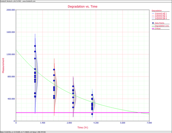
2. The following plot shows the degradation curve vs. time

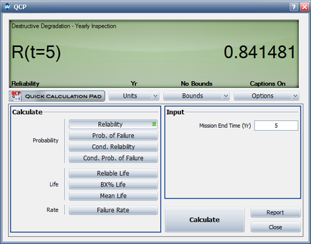
3. Using the QCP, the reliability at 5 years, or in other words the probability that the degradation measurement will be less than 150 at 5 years, is: