AND Gate

This page describes the AND gate and it's applications in Fault Tree diagrams used in Reliability and Safety Engineering.

In an AND gate, the output event occurs if all input events occur (or event A AND event B AND event C). When used in reliability and safety engineering an event is usualy a failure, a failure mode, or other undesirable event.

If one is looking at system reliability with each event represnting a component of the system then this this implies that all components must fail (input) in order for the system to fail (output). When using RBDs, the equivalent is a simple parallel configuration.

System Reliability Example

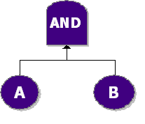
Consider a system with two components, A and B. The system fails if both A and B fail. Then the fault tree diagram is an AND gate (represinting the system level) with two events A and B. This is shown in the next figure.

Assuming independence then the reliability equation for either configuration is:

[math]\displaystyle{ {{R}_{System}}={{R}_{A}}+{{R}_{B}}-{{R}_{A}}\cdot {{R}_{B}} }[/math]

If we assume that the Relaibility of A is 0.90 and of B 0.85 then

[math]\displaystyle{ {{R}_{System}}=0.90+0.85-0.90\cdot 0.85 }[/math]

[math]\displaystyle{ {{R}_{System}}=0.985 }[/math]

Reliability deals with the probability of an event not occuring (the event being probability of failure of A, or Q(A)=P(A)), then if we are dealing directly with probabilities then P(A and B) = P(A ∩ B) = P(A) P(B).

[math]\displaystyle{ {{Q}_{System}}={{Q}_{A}}\cdot {{Q}_{B}} }[/math]

or

[math]\displaystyle{ {{Q}_{System}}=(1-0.90)\cdot (1-0.85) }[/math]

[math]\displaystyle{ {{Q}_{System}}=(0.015 }[/math].

Recall that

[math]\displaystyle{ {{R}_{System}}=1-{{Q}_{System}} }[/math]

[math]\displaystyle{ {{R}_{System}}=1-{0.015}=0.985. }[/math].

Failure Modes

The same can be expanded to failure modes. Consider a component that can fail due to failure modes, A and B and that the component will only fail if both modes occur. Then the probaility of failure is again

[math]\displaystyle{ {{Q}_{System}}={{Q}_{A}}\cdot {{Q}_{B}} }[/math]

Using Time Varying Formulations

Traditional fault trees defined events using a single constant probability. This concept can be easily expanded to probility distributions.

Consider again the prior system with two components, A and B. The system fails if both A and B fail.

Assuming independence then the reliability equation for either configuration is:

Furthermore assume that the reliability of each component is given by a reliability distribution R(t). Then

[math]\displaystyle{ {{R(t)}_{System}}={{R(t)}_{A}}+{{R(t)}_{B}}-{{R(t)}_{A}}\cdot {{R(t)}_{B}} }[/math].

If each of the components followed a e-parameter Weibull distribution or

[math]\displaystyle{ R(t)_A=e^{-\left( { \frac{t-\gamma_A }{\eta_A }}\right) ^{\beta_A }} }[/math]

[math]\displaystyle{ R(t)_B=e^{-\left( { \frac{t-\gamma_B }{\eta_B }}\right) ^{\beta_B }} }[/math]

then

[math]\displaystyle{ {{R(t)}_{System}}=e^{-\left( { \frac{t-\gamma_A }{\eta_A }}\right) ^{\beta_A }} +e^{-\left( { \frac{t-\gamma_B }{\eta_B }}\right) ^{\beta_B }} -e^{-\left( { \frac{t-\gamma_A }{\eta_A }}\right) ^{\beta_A }}\cdot e^{-\left( { \frac{t-\gamma_B }{\eta_B }}\right) ^{\beta_B }} }[/math]