|
|
| Line 1: |
Line 1: |
| {{InProgress}}
| |
| {{Reference Example}} | | {{Reference Example}} |
|
| |
|
Revision as of 21:11, 30 June 2015
New format available! This reference is now available in a new format that offers faster page load, improved display for calculations and images and more targeted search.
As of January 2024, this Reliawiki page will not continue to be updated. Please update all links and bookmarks to the latest references at Weibull examples and Weibull reference examples.
|
1P-Exponential MLE Solution for Interval Data
|
Compares the MLE solution, likelihood ratio bound and Fisher Matrix bound for a 1-parameter exponential distribution with interval data.
Reference Case
Example 7.1 on page 154 in the book Statistical Methods for Reliability Data by Dr. Meeker and Dr. Escobar, John Wiley & Sons, 1998. The sample size of 200 data is used here.
Data
| Number in State
|
Last Inspected
|
State F/S
|
State End Time
|
| 41 |
0 |
F |
100
|
| 44 |
100 |
F |
300
|
| 24 |
300 |
F |
500
|
| 32 |
500 |
F |
700
|
| 29 |
700 |
F |
1000
|
| 21 |
1000 |
F |
2000
|
| 9 |
2000 |
F |
4000
|
Result
The cumulative distribution function for an exponential distribution is:
- [math]\displaystyle{ F(t)=1-e^{-\left( \frac{t}{\theta }\right )}\,\! }[/math]
The ML estimate [math]\displaystyle{ \hat{\theta}\,\! }[/math] = 572.3, and the standard deviation is [math]\displaystyle{ se_{\hat\theta}\,\! }[/math] = 41.72. Therefore the variance is 1740.56.
The 95% 2-sided confidence interval for [math]\displaystyle{ {\theta}\,\! }[/math] are:
- Based on the likelihood ratio, the confidence interval is [498, 662]. The calculation is based on
- [math]\displaystyle{ -2ln\left [ \frac{L(\theta)}{L(\hat{\theta})} \right ] = X^{2}_{(0.90,1)}\,\! }[/math]
- The two solutions of [math]\displaystyle{ \theta\,\! }[/math] in the above equation will be the confidence bounds for [math]\displaystyle{ \theta\,\! }[/math].
- Based on lognormal approximation, the confidence interval is [496, 660]. The calculation is:
- [math]\displaystyle{ \begin{alignat}{2}
[\theta_{L},\theta_{U}]&= \hat{\theta}exp\left(\pm 1.96\times \frac{se_{\hat{\theta}}}{\hat{\theta}}\right)\\
&= \left[572.3\times exp \left(-1.96\times\frac{41.72}{572.3}\right),572.3\times exp \left(1.96\times\frac{41.72}{572.3}\right)\right]\\
&= [496,660]\\
\end{alignat} }[/math]
Results in Weibull++
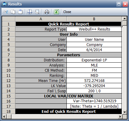
The ML estimator for [math]\displaystyle{ \theta\,\! }[/math] and its variance are 572.27 and 1740.52, respectively. They are given below.
The ML estimator for [math]\displaystyle{ \theta\,\! }[/math] and the variance are the same as the values given in the book.
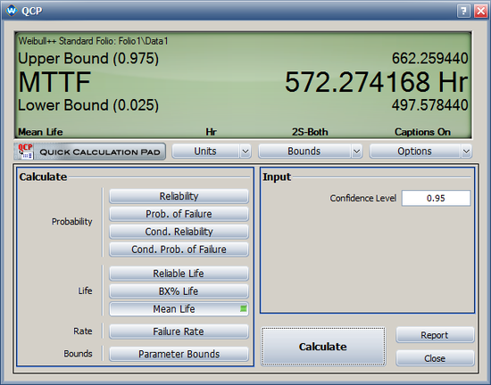
The 95% 2-sided confidence interval for [math]\displaystyle{ \theta\,\! }[/math] are:
- Based on the likelihood ratio (Select LRB for the confidence bound), the confidence interval is:
- Based on lognormal approximation (select FM for the bound method), the confidence bounds are:


