Cumulative Damage Model for Step Stress Profiles: Difference between revisions
Jump to navigation
Jump to search
Kate Racaza (talk | contribs) No edit summary |
Kate Racaza (talk | contribs) No edit summary |
||
| Line 372: | Line 372: | ||
| 9||100||102||36||27||1.333333||0.287682072||0.031977014 | | 9||100||102||36||27||1.333333||0.287682072||0.031977014 | ||
|- | |- | ||
| | |colspan="7" style="text-align:right;"|'''A ='''||0.132138165 | ||
|- | |- | ||
|} | |} | ||
The total cumulative damage at failure time of 102 is '''A''' in the above table. | The total cumulative damage at a failure time of 102 is '''A''' in the above table. | ||
Since the reliability function is: | Since the reliability function is: | ||
| Line 385: | Line 385: | ||
The probability density function (pdf) at time t is: | The probability density function (pdf) at time ''t'' is: | ||
::<math>\begin{align} | ::<math>\begin{align} | ||
| Line 404: | Line 404: | ||
Take | Take the logarithm of the above value and we get the log likelihood value for the first observation as <math>log(0.016) = -4.1489\,\!</math>. | ||
Repeating the above procedure, we can get the log likelihood value for each observation as given in the following table. | Repeating the above procedure, we can get the log likelihood value for each observation, as given in the following table. | ||
{| {{table}} | |||
! Status F/S||Time To F/S||Profile||Log likelihood Value | |||
|- | |||
| F||102||G1||-4.148929577 | |||
|- | |||
| F||113||G1||-4.518387096 | |||
|- | |||
| F||113||G1||-4.518387096 | |||
|- | |||
| S||370||G2||-0.72559186 | |||
|- | |||
| F||345||G2||-4.983506849 | |||
|- | |||
| S||345||G3||-0.910644661 | |||
|- | |||
| F||1249||G4||-6.199936981 | |||
|- | |||
| F||1333||G4||-7.129057207 | |||
|- | |||
| S||1333||G4||-2.451259934 | |||
|- | |||
| F||1096.6||G4||-6.518744419 | |||
|- | |||
| F||1250.8||G5||-6.075214111 | |||
|- | |||
| F||1097.9||G4||-6.523803805 | |||
|- | |||
| F||2460.9||G6||-8.444820079 | |||
|- | |||
| S||2460.9||G6||-0.29378846 | |||
|- | |||
| F||2700.4||G6||-8.566484581 | |||
|- | |||
| F||2923.9||G6||-7.469922325 | |||
|- | |||
| F||1160||G6||-9.119207934 | |||
|- | |||
| F||1962.9||G6||-8.086491838 | |||
|- | |||
| S||363.9||G6||-0.015237126 | |||
|- | |||
| F||898.4||G6||-10.4367511 | |||
|- | |||
| F||4142.1||G6||-7.897236924 | |||
|- | |||
|colspan = "3" style="text-align: right;"|'''Total'''||-115.033404 | |||
|- | |||
|} | |||
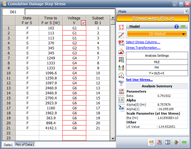
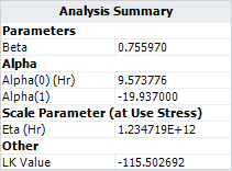
The log likelihood value calculated by hand in Excel is -115.0334, as given in the above table. It matches the value in ALTA. The slight difference is caused by the precision error. Therefore, the log likelihood value calculated in ALTA is correct. | |||
In fact, the optimization tool “Solver” in Excel can also be used to find the ML solutions. Using “Solver” and the “GRG” nonlinear optimization, we get the same results in Excel as in ALTA. | |||
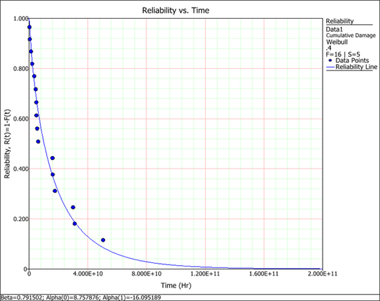
The following reliability plot shows that the predicted values (the line) by the model can match the observed values (the points) very well. | |||
[[Image:Step Stress_plot.png|center|550 px]] | |||
Revision as of 20:16, 16 June 2014
New format available! This reference is now available in a new format that offers faster page load, improved display for calculations and images and more targeted search.
As of January 2024, this Reliawiki page will not continue to be updated. Please update all links and bookmarks to the latest references at ALTA examples and ALTA reference examples.

