Crow-AMSAA Model - Helicopter System Example: Difference between revisions
mNo edit summary |
mNo edit summary |
||
| Line 93: | Line 93: | ||
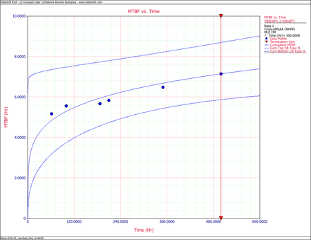
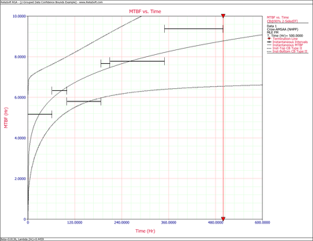
The next two figures show plots of the Fisher Matrix confidence bounds for the cumulative and instantaneous MTBF. | The next two figures show plots of the Fisher Matrix confidence bounds for the cumulative and instantaneous MTBF. | ||
[[Image:rga5.10.png|center| | [[Image:rga5.10.png|center|450px]] | ||
[[Image:rga5.11.png|center| | [[Image:rga5.11.png|center|450px]] | ||
The Crow confidence bounds for the cumulative and instantaneous MTBF at the 90% 2-sided confidence level and for <math>T = 500\,\!</math>hours are: | The Crow confidence bounds for the cumulative and instantaneous MTBF at the 90% 2-sided confidence level and for <math>T = 500\,\!</math>hours are: | ||
| Line 117: | Line 117: | ||
The next two figures show plots of the Crow confidence bounds for the cumulative and instantaneous MTBF. | The next two figures show plots of the Crow confidence bounds for the cumulative and instantaneous MTBF. | ||
[[Image:rga5.12.png|center| | [[Image:rga5.12.png|center|450px]] | ||
[[Image:rga5.13.png|center| | [[Image:rga5.13.png|center|450px]] | ||
</li> | </li> | ||
</ol> | </ol> | ||
Revision as of 18:34, 30 May 2014
New format available! This reference is now available in a new format that offers faster page load, improved display for calculations and images and more targeted search.
As of January 2024, this Reliawiki page will not continue to be updated. Please update all links and bookmarks to the latest references at RGA examples and RGA reference examples.
This example appears in the Reliability Growth and Repairable System Analysis Reference.
A new helicopter system is under development. System failure data has been collected on five helicopters during the final test phase. The actual failure times cannot be determined since the failures are not discovered until after the helicopters are brought into the maintenance area. However, total flying hours are known when the helicopters are brought in for service, and every 2 weeks each helicopter undergoes a thorough inspection to uncover any failures that may have occurred since the last inspection. Therefore, the cumulative total number of flight hours and the cumulative total number of failures for the 5 helicopters are known for each 2-week period. The total number of flight hours from the test phase is 500, which was accrued over a period of 12 weeks (six 2-week intervals). For each 2-week interval, the total number of flight hours and total number of failures for the 5 helicopters were recorded. The grouped data set is displayed in the following table.
| Interval | Interval Length | Failures in Interval |
|---|---|---|
| 1 | 0 - 62 | 12 |
| 2 | 62 -100 | 6 |
| 3 | 100 - 187 | 15 |
| 4 | 187 - 210 | 3 |
| 5 | 210 - 350 | 18 |
| 6 | 350 - 500 | 16 |
Do the following:
- Estimate the parameters of the Crow-AMSAA model using maximum likelihood estimation.
- Calculate the confidence bounds on the cumulative and instantaneous MTBF using the Fisher Matrix and Crow methods.
Solution
- Using RGA, the value of [math]\displaystyle{ \hat{\beta }\,\! }[/math], must be solved numerically. Once [math]\displaystyle{ \hat{\beta }\,\! }[/math] has been estimated then the value of [math]\displaystyle{ \hat{\lambda }\,\! }[/math] can be determined. The parameter values are displayed below:
- [math]\displaystyle{ \hat{\beta }= 0.81361\,\! }[/math]
- [math]\displaystyle{ \hat{\lambda }= 0.44585\,\! }[/math]
- [math]\displaystyle{ \begin{align} {{\beta }_{L}} = & \hat{\beta }{{e}^{{{z}_{\alpha }}\sqrt{Var(\hat{\beta })}/\hat{\beta }}} \\ = & 0.6546 \\ {{\beta }_{U}} = & \hat{\beta }{{e}^{-{{z}_{\alpha }}\sqrt{Var(\hat{\beta })}/\hat{\beta }}} \\ = & 1.0112 \end{align}\,\! }[/math]
- [math]\displaystyle{ \begin{align} {{\lambda }_{L}} = & \hat{\lambda }{{e}^{{{z}_{\alpha }}\sqrt{Var(\hat{\lambda })}/\hat{\lambda }}} \\ = & 0.14594 \\ {{\lambda }_{U}} = & \hat{\lambda }{{e}^{-{{z}_{\alpha }}\sqrt{Var(\hat{\lambda })}/\hat{\lambda }}} \\ = & 1.36207 \end{align}\,\! }[/math]
- [math]\displaystyle{ \begin{align} {{\beta }_{L}} = & \hat{\beta }(1-S) \\ = & 0.63552 \\ {{\beta }_{U}} = & \hat{\beta }(1+S) \\ = & 0.99170 \end{align}\,\! }[/math]
- [math]\displaystyle{ \begin{align} {{\lambda }_{L}} = & \frac{\chi _{\tfrac{\alpha }{2},2N}^{2}}{2\cdot T_{k}^{\beta }} \\ = & 0.36197 \\ {{\lambda }_{U}} = & \frac{\chi _{1-\tfrac{\alpha }{2},2N+2}^{2}}{2\cdot T_{k}^{\beta }} \\ = & 0.53697 \end{align}\,\! }[/math]
- The Fisher Matrix confidence bounds for the cumulative MTBF and the instantaneous MTBF at the 90% 2-sided confidence level and for [math]\displaystyle{ T=500\,\! }[/math] hour are:
- [math]\displaystyle{ \begin{align} {{[{{m}_{c}}(T)]}_{L}} = & {{{\hat{m}}}_{c}}(t){{e}^{{{z}_{\alpha /2}}\sqrt{Var({{{\hat{m}}}_{c}}(t))}/{{{\hat{m}}}_{c}}(t)}} \\ = & 5.8680 \\ {{[{{m}_{c}}(T)]}_{U}} = & {{{\hat{m}}}_{c}}(t){{e}^{-{{z}_{\alpha /2}}\sqrt{Var({{{\hat{m}}}_{c}}(t))}/{{{\hat{m}}}_{c}}(t)}} \\ = & 8.6947 \end{align}\,\! }[/math]
- [math]\displaystyle{ \begin{align} {{[MTB{{F}_{i}}]}_{L}} = & {{{\hat{m}}}_{i}}(t){{e}^{{{z}_{\alpha /2}}\sqrt{Var({{{\hat{m}}}_{i}}(t))}/{{{\hat{m}}}_{i}}(t)}} \\ = & 6.6483 \\ {{[MTB{{F}_{i}}]}_{U}} = & {{{\hat{m}}}_{i}}(t){{e}^{-{{z}_{\alpha /2}}\sqrt{Var({{{\hat{m}}}_{i}}(t))}/{{{\hat{m}}}_{i}}(t)}} \\ = & 11.5932 \end{align}\,\! }[/math]
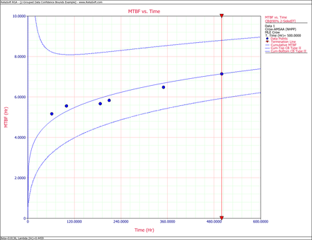
The Crow confidence bounds for the cumulative and instantaneous MTBF at the 90% 2-sided confidence level and for [math]\displaystyle{ T = 500\,\! }[/math]hours are:
- [math]\displaystyle{ \begin{align} {{[{{m}_{c}}(T)]}_{L}} = & \frac{1}{C{{(t)}_{U}}} \\ = & 5.85449 \\ {{[{{m}_{c}}(T)]}_{U}} = & \frac{1}{C{{(t)}_{L}}} \\ = & 8.79822 \end{align}\,\! }[/math]
and:
- [math]\displaystyle{ \begin{align} {{[MTB{{F}_{i}}]}_{L}} = & {{\hat{m}}_{i}}(1-W) \\ = & 6.19623 \\ {{[MTB{{F}_{i}}]}_{U}} = & {{\hat{m}}_{i}}(1+W) \\ = & 11.36223 \end{align}\,\! }[/math]
The next two figures show plots of the Crow confidence bounds for the cumulative and instantaneous MTBF.


