Crow-AMSAA Confidence Bounds Example: Difference between revisions
Chris Kahn (talk | contribs) No edit summary |
mNo edit summary |
||
| Line 10: | Line 10: | ||
The partial derivatives for the Fisher Matrix confidence bounds are: | The partial derivatives for the Fisher Matrix confidence bounds are: | ||
:<math>\begin{align} | :<math>\begin{align} | ||
| Line 17: | Line 16: | ||
\frac{{{\partial }^{2}}\Lambda }{\partial \lambda \partial \beta } = & -{{620}^{0.6142}}\ln 620=-333.64 | \frac{{{\partial }^{2}}\Lambda }{\partial \lambda \partial \beta } = & -{{620}^{0.6142}}\ln 620=-333.64 | ||
\end{align}\,\!</math> | \end{align}\,\!</math> | ||
The Fisher Matrix then becomes: | The Fisher Matrix then becomes: | ||
:<math>\begin{align} | :<math>\begin{align} | ||
| Line 27: | Line 24: | ||
& = \begin{bmatrix} 0.13519969 & -0.046614609\\ -0.046614609 & 0.017105343 \end{bmatrix} | & = \begin{bmatrix} 0.13519969 & -0.046614609\\ -0.046614609 & 0.017105343 \end{bmatrix} | ||
\end{align}\,\!</math> | \end{align}\,\!</math> | ||
For <math>T=620\,\!</math> hours, the partial derivatives of the cumulative and instantaneous failure intensities are: | For <math>T=620\,\!</math> hours, the partial derivatives of the cumulative and instantaneous failure intensities are: | ||
:<math>\begin{align} | :<math>\begin{align} | ||
| Line 40: | Line 35: | ||
= & 0.083694185 | = & 0.083694185 | ||
\end{align}\,\!</math> | \end{align}\,\!</math> | ||
:<math>\begin{align} | :<math>\begin{align} | ||
| Line 47: | Line 41: | ||
= & 0.17558519 | = & 0.17558519 | ||
\end{align}\,\!</math> | \end{align}\,\!</math> | ||
:<math>\begin{align} | :<math>\begin{align} | ||
| Line 54: | Line 47: | ||
= & 0.051404969 | = & 0.051404969 | ||
\end{align}\,\!</math> | \end{align}\,\!</math> | ||
Therefore, the variances become: | Therefore, the variances become: | ||
:<math>\begin{align} | :<math>\begin{align} | ||
| Line 65: | Line 56: | ||
&= 0.0000431393 | &= 0.0000431393 | ||
\end{align}\,\!</math> | \end{align}\,\!</math> | ||
The cumulative and instantaneous failure intensities at <math>T=620\,\!</math> hours are: | The cumulative and instantaneous failure intensities at <math>T=620\,\!</math> hours are: | ||
:<math>\begin{align} | :<math>\begin{align} | ||
| Line 74: | Line 63: | ||
{{\lambda }_{i}}(T)= & 0.02179 | {{\lambda }_{i}}(T)= & 0.02179 | ||
\end{align}\,\!</math> | \end{align}\,\!</math> | ||
So, at the 90% confidence level and for <math>T=620\,\!</math> hours, the Fisher Matrix confidence bounds for the cumulative failure intensity are: | So, at the 90% confidence level and for <math>T=620\,\!</math> hours, the Fisher Matrix confidence bounds for the cumulative failure intensity are: | ||
:<math>\begin{align} | :<math>\begin{align} | ||
| Line 83: | Line 70: | ||
{{[{{\lambda }_{c}}(T)]}_{U}}= & 0.05039 | {{[{{\lambda }_{c}}(T)]}_{U}}= & 0.05039 | ||
\end{align}\,\!</math> | \end{align}\,\!</math> | ||
The confidence bounds for the instantaneous failure intensity are: | The confidence bounds for the instantaneous failure intensity are: | ||
:<math>\begin{align} | :<math>\begin{align} | ||
| Line 92: | Line 77: | ||
{{[{{\lambda }_{i}}(T)]}_{U}}= & 0.03579 | {{[{{\lambda }_{i}}(T)]}_{U}}= & 0.03579 | ||
\end{align}\,\!</math> | \end{align}\,\!</math> | ||
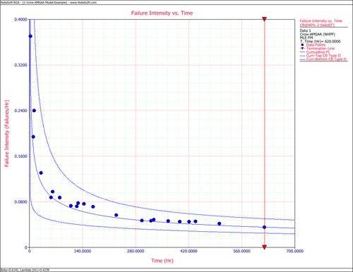
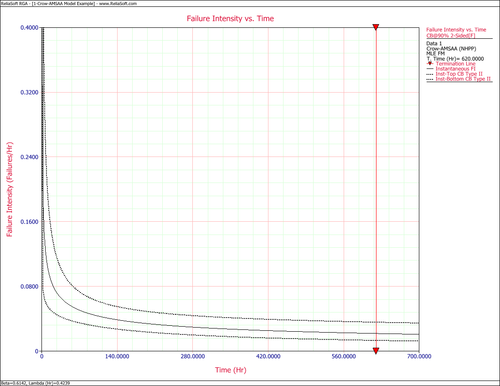
The following figures display plots of the Fisher Matrix confidence bounds for the cumulative and instantaneous failure intensity, respectively. | The following figures display plots of the Fisher Matrix confidence bounds for the cumulative and instantaneous failure intensity, respectively. | ||
[[Image:rga5.2.png|center|500px|Cumulative failure intensity with 2-sided 90% Fisher Matrix confidence bounds.]] | [[Image:rga5.2.png|center|500px|Cumulative failure intensity with 2-sided 90% Fisher Matrix confidence bounds.]] | ||
| Line 101: | Line 84: | ||
[[Image:rga5.3.png|center|500px|Instantaneous failure intensity with 2-sided 90% Fisher Matrix confidence bounds.]] | [[Image:rga5.3.png|center|500px|Instantaneous failure intensity with 2-sided 90% Fisher Matrix confidence bounds.]] | ||
'''Crow Bounds''' | '''Crow Bounds''' | ||
Given that the data is failure terminated, the Crow confidence bounds for the cumulative failure intensity at the 90% confidence level and for <math>T=620\,\!</math> hours are: | Given that the data is failure terminated, the Crow confidence bounds for the cumulative failure intensity at the 90% confidence level and for <math>T=620\,\!</math> hours are: | ||
:<math>\begin{align} | :<math>\begin{align} | ||
| Line 116: | Line 97: | ||
= & 0.048775 | = & 0.048775 | ||
\end{align}\,\!</math> | \end{align}\,\!</math> | ||
The Crow confidence bounds for the instantaneous failure intensity at the 90% confidence level and for <math>T=620\,\!</math> hours are calculated by first estimating the bounds on the instantaneous MTBF. Once these are calculated, take the inverse as shown below. Details on the confidence bounds for instantaneous MTBF are presented [[Crow-AMSAA Confidence Bounds#Crow_Bounds_4|here]]. | The Crow confidence bounds for the instantaneous failure intensity at the 90% confidence level and for <math>T=620\,\!</math> hours are calculated by first estimating the bounds on the instantaneous MTBF. Once these are calculated, take the inverse as shown below. Details on the confidence bounds for instantaneous MTBF are presented [[Crow-AMSAA Confidence Bounds#Crow_Bounds_4|here]]. | ||
:<math>\begin{align} | :<math>\begin{align} | ||
| Line 126: | Line 105: | ||
= & 0.01179 | = & 0.01179 | ||
\end{align}\,\!</math> | \end{align}\,\!</math> | ||
:<math>\begin{align} | :<math>\begin{align} | ||
| Line 133: | Line 111: | ||
= & 0.03253 | = & 0.03253 | ||
\end{align}\,\!</math> | \end{align}\,\!</math> | ||
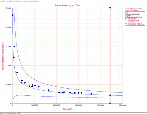
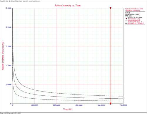
The following figures display plots of the Crow confidence bounds for the cumulative and instantaneous failure intensity, respectively. | The following figures display plots of the Crow confidence bounds for the cumulative and instantaneous failure intensity, respectively. | ||
[[Image:rga5.4.png|center|500px|Cumulative failure intensity with 2-sided 90% Crow confidence bounds.]] | [[Image:rga5.4.png|center|500px|Cumulative failure intensity with 2-sided 90% Crow confidence bounds.]] | ||
| Line 142: | Line 118: | ||
[[Image:rga5.5.png|center|500px|Instantaneous failure intensity with 2-sided 90% Crow confidence bounds.]] | [[Image:rga5.5.png|center|500px|Instantaneous failure intensity with 2-sided 90% Crow confidence bounds.]] | ||
====Failure Times - Example 3==== | ====Failure Times - Example 3==== | ||
| Line 152: | Line 127: | ||
From the previous example: | From the previous example: | ||
:<math>\begin{align} | :<math>\begin{align} | ||
| Line 159: | Line 133: | ||
Cov(\hat{\beta },\hat{\lambda }) = & -0.046614609 | Cov(\hat{\beta },\hat{\lambda }) = & -0.046614609 | ||
\end{align}\,\!</math> | \end{align}\,\!</math> | ||
And for <math>T=620\,\!</math> hours, the partial derivatives of the cumulative and instantaneous MTBF are: | And for <math>T=620\,\!</math> hours, the partial derivatives of the cumulative and instantaneous MTBF are: | ||
:<math>\begin{align} | :<math>\begin{align} | ||
| Line 178: | Line 150: | ||
= & -108.26001 | = & -108.26001 | ||
\end{align}\,\!</math> | \end{align}\,\!</math> | ||
Therefore, the variances become: | Therefore, the variances become: | ||
:<math>\begin{align} | :<math>\begin{align} | ||
| Line 188: | Line 158: | ||
= & 36.113376 | = & 36.113376 | ||
\end{align}\,\!</math> | \end{align}\,\!</math> | ||
:<math>\begin{align} | :<math>\begin{align} | ||
| Line 195: | Line 164: | ||
= & 191.33709 | = & 191.33709 | ||
\end{align}\,\!</math> | \end{align}\,\!</math> | ||
So, at 90% confidence level and <math>T=620\,\!</math> hours, the Fisher Matrix confidence bounds are: | So, at 90% confidence level and <math>T=620\,\!</math> hours, the Fisher Matrix confidence bounds are: | ||
:<math>\begin{align} | :<math>\begin{align} | ||
| Line 206: | Line 173: | ||
= & 40.01927 | = & 40.01927 | ||
\end{align}\,\!</math> | \end{align}\,\!</math> | ||
:<math>\begin{align} | :<math>\begin{align} | ||
| Line 214: | Line 180: | ||
= & 75.34193 | = & 75.34193 | ||
\end{align}\,\!</math> | \end{align}\,\!</math> | ||
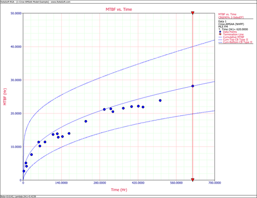
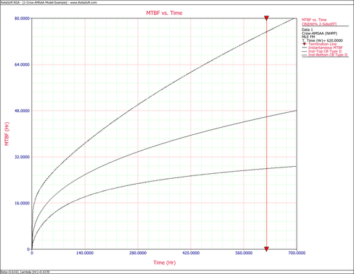
The following two figures show plots of the Fisher Matrix confidence bounds for the cumulative and instantaneous MTBFs. | The following two figures show plots of the Fisher Matrix confidence bounds for the cumulative and instantaneous MTBFs. | ||
[[Image:rga5.6.png|center|500px|Cumulative MTBF with 2-sided 90% Fisher Matrix confidence bounds.]] | [[Image:rga5.6.png|center|500px|Cumulative MTBF with 2-sided 90% Fisher Matrix confidence bounds.]] | ||
| Line 223: | Line 187: | ||
[[Image:rga5.7.png|center|500px|Instantaneous MTBF with 2-sided Fisher Matrix confidence bounds.]] | [[Image:rga5.7.png|center|500px|Instantaneous MTBF with 2-sided Fisher Matrix confidence bounds.]] | ||
'''Crow Bounds''' | '''Crow Bounds''' | ||
The Crow confidence bounds for the cumulative MTBF and the instantaneous MTBF at the 90% confidence level and for <math>T=620\,\!</math> hours are: | The Crow confidence bounds for the cumulative MTBF and the instantaneous MTBF at the 90% confidence level and for <math>T=620\,\!</math> hours are: | ||
:<math>\begin{align} | :<math>\begin{align} | ||
| Line 236: | Line 198: | ||
= & 41.6282 | = & 41.6282 | ||
\end{align}\,\!</math> | \end{align}\,\!</math> | ||
:<math>\begin{align} | :<math>\begin{align} | ||
| Line 244: | Line 205: | ||
= & 84.7972 | = & 84.7972 | ||
\end{align}\,\!</math> | \end{align}\,\!</math> | ||
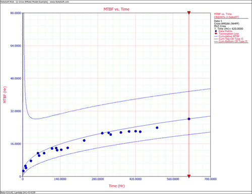
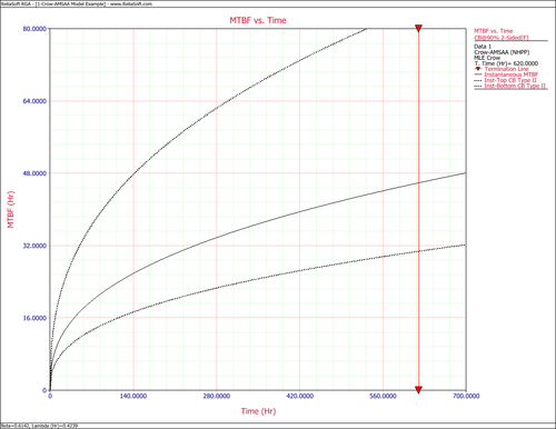
The figures below show plots of the Crow confidence bounds for the cumulative and instantaneous MTBF. | The figures below show plots of the Crow confidence bounds for the cumulative and instantaneous MTBF. | ||
| Line 254: | Line 214: | ||
Confidence bounds can also be obtained on the parameters <math>\hat{\beta }\,\!</math> and <math>\hat{\lambda }\,\!</math>. For Fisher Matrix confidence bounds: | Confidence bounds can also be obtained on the parameters <math>\hat{\beta }\,\!</math> and <math>\hat{\lambda }\,\!</math>. For Fisher Matrix confidence bounds: | ||
:<math>\begin{align} | :<math>\begin{align} | ||
| Line 262: | Line 221: | ||
= & 0.8722 | = & 0.8722 | ||
\end{align}\,\!</math> | \end{align}\,\!</math> | ||
and: | and: | ||
:<math>\begin{align} | :<math>\begin{align} | ||
| Line 273: | Line 230: | ||
= & 1.7691 | = & 1.7691 | ||
\end{align}\,\!</math> | \end{align}\,\!</math> | ||
For Crow confidence bounds: | For Crow confidence bounds: | ||
:<math>\begin{align} | :<math>\begin{align} | ||
| Line 282: | Line 237: | ||
{{\beta }_{U}}= & 0.9350 | {{\beta }_{U}}= & 0.9350 | ||
\end{align}\,\!</math> | \end{align}\,\!</math> | ||
and: | and: | ||
:<math>\begin{align} | :<math>\begin{align} | ||
Revision as of 20:46, 30 January 2014
New format available! This reference is now available in a new format that offers faster page load, improved display for calculations and images and more targeted search.
As of January 2024, this Reliawiki page will not continue to be updated. Please update all links and bookmarks to the latest references at RGA examples and RGA reference examples.
This example appears in the Reliability Growth and Repairable System Analysis Reference book.
Using the values of [math]\displaystyle{ \hat{\beta }\,\! }[/math] and [math]\displaystyle{ \hat{\lambda }\,\! }[/math] estimated in the Failure Times - Example 1, calculate the 90% 2-sided confidence bounds on the cumulative and instantaneous failure intensity.
Solution
Fisher Matrix Bounds
The partial derivatives for the Fisher Matrix confidence bounds are:
- [math]\displaystyle{ \begin{align} \frac{{{\partial }^{2}}\Lambda }{\partial {{\lambda }^{2}}} = & -\frac{22}{{{0.4239}^{2}}}=-122.43 \\ \frac{{{\partial }^{2}}\Lambda }{\partial {{\beta }^{2}}} = & -\frac{22}{{{0.6142}^{2}}}-0.4239\cdot {{620}^{0.6142}}{{(\ln 620)}^{2}}=-967.68 \\ \frac{{{\partial }^{2}}\Lambda }{\partial \lambda \partial \beta } = & -{{620}^{0.6142}}\ln 620=-333.64 \end{align}\,\! }[/math]
The Fisher Matrix then becomes:
- [math]\displaystyle{ \begin{align} \begin{bmatrix}122.43 & 333.64\\ 333.64 & 967.68\end{bmatrix}^{-1} & = \begin{bmatrix}Var(\hat{\lambda}) & Cov(\hat{\beta},\hat{\lambda})\\ Cov(\hat{\beta},\hat{\lambda}) & Var(\hat{\beta})\end{bmatrix} \\ & = \begin{bmatrix} 0.13519969 & -0.046614609\\ -0.046614609 & 0.017105343 \end{bmatrix} \end{align}\,\! }[/math]
For [math]\displaystyle{ T=620\,\! }[/math] hours, the partial derivatives of the cumulative and instantaneous failure intensities are:
- [math]\displaystyle{ \begin{align} \frac{\partial {{\lambda }_{c}}(T)}{\partial \beta }= & \hat{\lambda }{{T}^{\hat{\beta }-1}}\ln (T) \\ = & 0.4239\cdot {{620}^{-0.3858}}\ln 620 \\ = & 0.22811336 \\ \frac{\partial {{\lambda }_{c}}(T)}{\partial \lambda }= & {{T}^{\hat{\beta }-1}} \\ = & {{620}^{-0.3858}} \\ = & 0.083694185 \end{align}\,\! }[/math]
- [math]\displaystyle{ \begin{align} \frac{\partial {{\lambda }_{i}}(T)}{\partial \beta }= & \hat{\lambda }{{T}^{\hat{\beta }-1}}+\hat{\lambda }\hat{\beta }{{T}^{\hat{\beta }-1}}\ln T \\ = & 0.4239\cdot {{620}^{-0.3858}}+0.4239\cdot 0.6142\cdot {{620}^{-0.3858}}\ln 620 \\ = & 0.17558519 \end{align}\,\! }[/math]
- [math]\displaystyle{ \begin{align} \frac{\partial {{\lambda }_{i}}(T)}{\partial \lambda }= & \hat{\beta }{{T}^{\hat{\beta }-1}} \\ = & 0.6142\cdot {{620}^{-0.3858}} \\ = & 0.051404969 \end{align}\,\! }[/math]
Therefore, the variances become:
- [math]\displaystyle{ \begin{align} Var(\hat{\lambda_{c}}(T)) & = 0.22811336^{2}\cdot 0.017105343\ + 0.083694185^{2} \cdot 0.13519969\ -2\cdot 0.22811336\cdot 0.083694185\cdot 0.046614609 \\ & = 0.00005721408 \\ Var(\hat{\lambda_{i}}(T)) & = 0.17558519^{2}\cdot 0.01715343\ + 0.051404969^{2}\cdot 0.13519969\ -2\cdot 0.17558519\cdot 0.051404969\cdot 0.046614609 \\ &= 0.0000431393 \end{align}\,\! }[/math]
The cumulative and instantaneous failure intensities at [math]\displaystyle{ T=620\,\! }[/math] hours are:
- [math]\displaystyle{ \begin{align} {{\lambda }_{c}}(T)= & 0.03548 \\ {{\lambda }_{i}}(T)= & 0.02179 \end{align}\,\! }[/math]
So, at the 90% confidence level and for [math]\displaystyle{ T=620\,\! }[/math] hours, the Fisher Matrix confidence bounds for the cumulative failure intensity are:
- [math]\displaystyle{ \begin{align} {{[{{\lambda }_{c}}(T)]}_{L}}= & 0.02499 \\ {{[{{\lambda }_{c}}(T)]}_{U}}= & 0.05039 \end{align}\,\! }[/math]
The confidence bounds for the instantaneous failure intensity are:
- [math]\displaystyle{ \begin{align} {{[{{\lambda }_{i}}(T)]}_{L}}= & 0.01327 \\ {{[{{\lambda }_{i}}(T)]}_{U}}= & 0.03579 \end{align}\,\! }[/math]
The following figures display plots of the Fisher Matrix confidence bounds for the cumulative and instantaneous failure intensity, respectively.
Crow Bounds
Given that the data is failure terminated, the Crow confidence bounds for the cumulative failure intensity at the 90% confidence level and for [math]\displaystyle{ T=620\,\! }[/math] hours are:
- [math]\displaystyle{ \begin{align} {{[{{\lambda }_{c}}(T)]}_{L}} = & \frac{\chi _{\tfrac{\alpha }{2},2N}^{2}}{2\cdot t} \\ = & \frac{29.787476}{2*620} \\ = & 0.02402 \\ {{[{{\lambda }_{c}}(T)]}_{U}} = & \frac{\chi _{1-\tfrac{\alpha }{2},2N}^{2}}{2\cdot t} \\ = & \frac{60.48089}{2*620} \\ = & 0.048775 \end{align}\,\! }[/math]
The Crow confidence bounds for the instantaneous failure intensity at the 90% confidence level and for [math]\displaystyle{ T=620\,\! }[/math] hours are calculated by first estimating the bounds on the instantaneous MTBF. Once these are calculated, take the inverse as shown below. Details on the confidence bounds for instantaneous MTBF are presented here.
- [math]\displaystyle{ \begin{align} {{[{{\lambda }_{i}}(t)]}_{L}} = & \frac{1}{{{[MTB{{F}_{i}}]}_{U}}} \\ = & \frac{1}{MTB{{F}_{i}}\cdot U} \\ = & 0.01179 \end{align}\,\! }[/math]
- [math]\displaystyle{ \begin{align} {{[{{\lambda }_{i}}(t)]}_{U}}= & \frac{1}{{{[MTB{{F}_{i}}]}_{L}}} \\ = & \frac{1}{MTB{{F}_{i}}\cdot L} \\ = & 0.03253 \end{align}\,\! }[/math]
The following figures display plots of the Crow confidence bounds for the cumulative and instantaneous failure intensity, respectively.
Failure Times - Example 3
Calculate the confidence bounds on the cumulative and instantaneous MTBF for the data from the example given above.
Solution
Fisher Matrix Bounds
From the previous example:
- [math]\displaystyle{ \begin{align} Var(\hat{\lambda }) = & 0.13519969 \\ Var(\hat{\beta }) = & 0.017105343 \\ Cov(\hat{\beta },\hat{\lambda }) = & -0.046614609 \end{align}\,\! }[/math]
And for [math]\displaystyle{ T=620\,\! }[/math] hours, the partial derivatives of the cumulative and instantaneous MTBF are:
- [math]\displaystyle{ \begin{align} \frac{\partial {{m}_{c}}(T)}{\partial \beta }= & -\frac{1}{\hat{\lambda }}{{T}^{1-\hat{\beta }}}\ln T \\ = & -\frac{1}{0.4239}{{620}^{0.3858}}\ln 620 \\ = & -181.23135 \\ \frac{\partial {{m}_{c}}(T)}{\partial \lambda } = & -\frac{1}{{{\hat{\lambda }}^{2}}}{{T}^{1-\hat{\beta }}} \\ = & -\frac{1}{{{0.4239}^{2}}}{{620}^{0.3858}} \\ = & -66.493299 \\ \frac{\partial {{m}_{i}}(T)}{\partial \beta } = & -\frac{1}{\hat{\lambda }{{\hat{\beta }}^{2}}}{{T}^{1-\beta }}-\frac{1}{\hat{\lambda }\hat{\beta }}{{T}^{1-\hat{\beta }}}\ln T \\ = & -\frac{1}{0.4239\cdot {{0.6142}^{2}}}{{620}^{0.3858}}-\frac{1}{0.4239\cdot 0.6142}{{620}^{0.3858}}\ln 620 \\ = & -369.78634 \\ \frac{\partial {{m}_{i}}(T)}{\partial \lambda } = & -\frac{1}{{{\hat{\lambda }}^{2}}\hat{\beta }}{{T}^{1-\hat{\beta }}} \\ = & -\frac{1}{{{0.4239}^{2}}\cdot 0.6142}\cdot {{620}^{0.3858}} \\ = & -108.26001 \end{align}\,\! }[/math]
Therefore, the variances become:
- [math]\displaystyle{ \begin{align} Var({{\hat{m}}_{c}}(T)) = & {{\left( -181.23135 \right)}^{2}}\cdot 0.017105343+{{\left( -66.493299 \right)}^{2}}\cdot 0.13519969 \\ & -2\cdot \left( -181.23135 \right)\cdot \left( -66.493299 \right)\cdot 0.046614609 \\ = & 36.113376 \end{align}\,\! }[/math]
- [math]\displaystyle{ \begin{align} Var({{\hat{m}}_{i}}(T)) = & {{\left( -369.78634 \right)}^{2}}\cdot 0.017105343+{{\left( -108.26001 \right)}^{2}}\cdot 0.13519969 \\ & -2\cdot \left( -369.78634 \right)\cdot \left( -108.26001 \right)\cdot 0.046614609 \\ = & 191.33709 \end{align}\,\! }[/math]
So, at 90% confidence level and [math]\displaystyle{ T=620\,\! }[/math] hours, the Fisher Matrix confidence bounds are:
- [math]\displaystyle{ \begin{align} {{[{{m}_{c}}(T)]}_{L}} = & {{{\hat{m}}}_{c}}(t){{e}^{-{{z}_{\alpha }}\sqrt{Var({{{\hat{m}}}_{c}}(t))}/{{{\hat{m}}}_{c}}(t)}} \\ = & 19.84581 \\ {{[{{m}_{c}}(T)]}_{U}} = & {{{\hat{m}}}_{c}}(t){{e}^{{{z}_{\alpha }}\sqrt{Var({{{\hat{m}}}_{c}}(t))}/{{{\hat{m}}}_{c}}(t)}} \\ = & 40.01927 \end{align}\,\! }[/math]
- [math]\displaystyle{ \begin{align} {{[{{m}_{i}}(T)]}_{L}} = & {{{\hat{m}}}_{i}}(t){{e}^{-{{z}_{\alpha }}\sqrt{Var({{{\hat{m}}}_{i}}(t))}/{{{\hat{m}}}_{i}}(t)}} \\ = & 27.94261 \\ {{[{{m}_{i}}(T)]}_{U}} = & {{{\hat{m}}}_{i}}(t){{e}^{{{z}_{\alpha }}\sqrt{Var({{{\hat{m}}}_{i}}(t))}/{{{\hat{m}}}_{i}}(t)}} \\ = & 75.34193 \end{align}\,\! }[/math]
The following two figures show plots of the Fisher Matrix confidence bounds for the cumulative and instantaneous MTBFs.
Crow Bounds
The Crow confidence bounds for the cumulative MTBF and the instantaneous MTBF at the 90% confidence level and for [math]\displaystyle{ T=620\,\! }[/math] hours are:
- [math]\displaystyle{ \begin{align} {{[{{m}_{c}}(T)]}_{L}} = & \frac{1}{{{[{{\lambda }_{c}}(T)]}_{U}}} \\ = & 20.5023 \\ {{[{{m}_{c}}(T)]}_{U}} = & \frac{1}{{{[{{\lambda }_{c}}(T)]}_{L}}} \\ = & 41.6282 \end{align}\,\! }[/math]
- [math]\displaystyle{ \begin{align} {{[MTB{{F}_{i}}]}_{L}} = & MTB{{F}_{i}}\cdot {{\Pi }_{1}} \\ = & 30.7445 \\ {{[MTB{{F}_{i}}]}_{U}} = & MTB{{F}_{i}}\cdot {{\Pi }_{2}} \\ = & 84.7972 \end{align}\,\! }[/math]
The figures below show plots of the Crow confidence bounds for the cumulative and instantaneous MTBF.
Confidence bounds can also be obtained on the parameters [math]\displaystyle{ \hat{\beta }\,\! }[/math] and [math]\displaystyle{ \hat{\lambda }\,\! }[/math]. For Fisher Matrix confidence bounds:
- [math]\displaystyle{ \begin{align} {{\beta }_{L}} = & \hat{\beta }{{e}^{{{z}_{\alpha }}\sqrt{Var(\hat{\beta })}/\hat{\beta }}} \\ = & 0.4325 \\ {{\beta }_{U}} = & \hat{\beta }{{e}^{-{{z}_{\alpha }}\sqrt{Var(\hat{\beta })}/\hat{\beta }}} \\ = & 0.8722 \end{align}\,\! }[/math]
and:
- [math]\displaystyle{ \begin{align} {{\lambda }_{L}} = & \hat{\lambda }{{e}^{{{z}_{\alpha }}\sqrt{Var(\hat{\lambda })}/\hat{\lambda }}} \\ = & 0.1016 \\ {{\lambda }_{U}} = & \hat{\lambda }{{e}^{-{{z}_{\alpha }}\sqrt{Var(\hat{\lambda })}/\hat{\lambda }}} \\ = & 1.7691 \end{align}\,\! }[/math]
For Crow confidence bounds:
- [math]\displaystyle{ \begin{align} {{\beta }_{L}}= & 0.4527 \\ {{\beta }_{U}}= & 0.9350 \end{align}\,\! }[/math]
and:
- [math]\displaystyle{ \begin{align} {{\lambda }_{L}}= & 0.2870 \\ {{\lambda }_{U}}= & 0.5827 \end{align}\,\! }[/math]

