Simulation with RGA Models: Difference between revisions
| Line 126: | Line 126: | ||
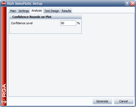
[[Image:rga14.9.png|thumb|center|450px|The '''Analysis''' tab of the SimuMatic window.]] | [[Image:rga14.9.png|thumb|center|450px|The '''Analysis''' tab of the SimuMatic window.]] | ||
[[Image:rga14.9.5.png|thumb|center|450px|The '''Test Design''' tab of the SimuMatic window.]] | |||
[[Image:rga14.10.png|thumb|center|450px|The '''Results''' tab of the SimuMatic window.]] | [[Image:rga14.10.png|thumb|center|450px|The '''Results''' tab of the SimuMatic window.]] | ||
Revision as of 19:33, 27 November 2013
When analyzing developmental systems for reliability growth, and conducting data analysis of fielded repairable systems, it is often useful to experiment with various what if scenarios or put together hypothetical analyses before data sets become available in order to plan for the best way to perform the analysis. With that in mind, the RGA software offers applications based on Monte Carlo simulation that can be used in order to:
- a) Better understand reliability growth concepts.
- b) Experiment with the impact of sample size, test time and growth parameters on analysis results.
- c) Construct simulation-based confidence intervals.
- d) Better understand concepts behind confidence intervals.
- e) Design reliability demonstration tests.
There are two applications of the Monte Carlo simulation in the RGA software. One is called Generate Monte Carlo Data and the other is called SimuMatic.
Generate Monte Carlo Data
Monte Carlo simulation is a computational algorithm in which we randomly generate input variables that follow a specified probability distribution. In the case of reliability growth and repairable system data analysis, we are interested in generating failure times for systems that we assume to have specific characteristics. In our applications we want the inter-arrival times of the failures to follow a non-homogeneous Poisson process with a Weibull failure intensity, as specified in the Crow-AMSAA (NHPP) model.
The first time to failure, [math]\displaystyle{ {{t}_{1}},\,\! }[/math] is assumed to follow a Weibull distribution. It is obtained by solving for [math]\displaystyle{ {{t}_{1}}\,\! }[/math] :
- [math]\displaystyle{ R(t_1)=e^{(-\frac{t_1}{\eta})^\beta}= Uniform (0,1)\,\! }[/math]
- where:
- [math]\displaystyle{ \eta ={{\left( \frac{1}{\lambda } \right)}^{\tfrac{1}{\beta }}}\,\! }[/math]
Solving for [math]\displaystyle{ {{t}_{1}}\,\! }[/math] yields:
- [math]\displaystyle{ t_{1} = \eta \left [ -ln(Uniform(0,1)) \right ]^{\frac {1}{\beta}} }[/math]
The failure times are then obtained based on the conditional unreliability equation that describes the non-homogeneous Poisson process (NHPP):
- [math]\displaystyle{ F(t_{i}\ | \ t_{i-1}) = 1 -e^{-\lambda\left[t_{i}^{\beta}-t_{i-1}^{\beta}\right]} = Uniform(0,1) }[/math]
and then solving for [math]\displaystyle{ {{t}_{i}}\,\! }[/math] yields:
- [math]\displaystyle{ t_{i}=\left[-\frac {ln(1-Uniform(0,1))}{\lambda}+t_{i-1}^{\beta} \right ]^{\frac{1}{\beta}} }[/math]
To access the data generation utility, choose Home > Tools > Generate Monte Carlo Data. There are different data types that can be generated with the Monte Carlo utility. For all of them, the basic parameters that are always specified are the beta [math]\displaystyle{ (\beta )\,\! }[/math] and lambda [math]\displaystyle{ (\lambda )\,\! }[/math] parameters of the Crow-AMSAA (NHPP) model. That does not mean that the generated data can be analyzed only with the Crow-AMSAA (NHPP) model. Depending on the data type, the Duane, Crow extended and power law models can also be used. They share the same growth patterns, which are based on the [math]\displaystyle{ \beta \,\! }[/math] and [math]\displaystyle{ \lambda \,\! }[/math] parameters. In the case of the Duane model, [math]\displaystyle{ \beta =1-\alpha \,\! }[/math], where [math]\displaystyle{ \alpha \,\! }[/math] is the growth parameter for the Duane model. Below we present the available data types that can generated with the Monte Carlo utility.
- Failure Times: The data set is generated assuming a single system. There is a choice between a time terminated test, where the termination time needs to be specified, or a failure terminated test, where the number of failures needs to be specified. The generated failure times data can then be analyzed using the Duane or Crow-AMSAA (NHPP) models, or the Crow extended model if classifications and modes are entered for the failures.
- Grouped Failure Times: The data is generated assuming a single system. There is a choice between a time terminated test, where the termination time needs to be specified, or a failure terminated test, where the number of failures needs to be specified. In addition, constant or user-defined intervals need to be specified for the grouping of the data. The generated grouped data can then be analyzed using the Duane or Crow-AMSAA (NHPP) models, or the Crow Extended model if classifications and modes are entered for the failures.
- Multiple Systems - Concurrent: In this case, the number of systems needs to be specified. There is a choice between a time terminated test, where the termination time needs to be specified, or a failure terminated test, where the number of failures needs to be specified. The generated folio contains failure times for each of the systems. The data can then be analyzed using the Duane or Crow-AMSAA (NHPP) models, or the Crow Extended model if classifications and modes are entered for the failures.
- Repairable Systems: In this case, the number of systems needs to be specified. There is a choice between a time terminated test, where the termination time needs to be specified, or a failure terminated test, where the number of failures needs to be specified. The generated folio contains failure times for each of the systems. The data can then be analyzed using the power law model, or the Crow extended model if classifications and modes are entered for the failures.
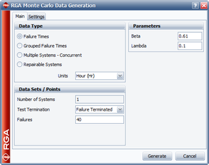
The next figure shows the Monte Carlo utility and all the necessary user inputs.
The seed determines the starting point from which the random numbers will be generated. The use of a seed forces the software to use the same sequence of random numbers, resulting in repeatability. In other words, the same failure times can be generated if the same seed, data type, parameters and number of points/systems are used. If no seed is provided, the computer's clock is used to initialize the random number generator and a different set of failure times will be generated at each new request.
Monte Carlo Data Example
A reliability engineer wants to experiment with different testing scenarios as the reliability growth test of the company's new product is being prepared. From the reliability growth test data of a similar product that was developed previously, the beta and lambda parameters are [math]\displaystyle{ \beta =0.5\,\! }[/math] and [math]\displaystyle{ \lambda =0.75.\,\! }[/math] Three systems are to be used to generate a representative data set of expected times-to-failure for the upcoming test. The purpose is to explore different test durations in order to demonstrate an MTBF of 200 hours.
Solution
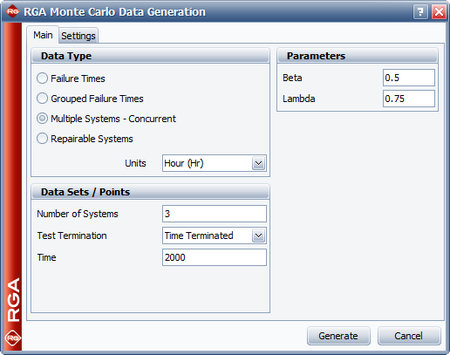
In the Monte Carlo window, the parameters are set to [math]\displaystyle{ \beta =0.5\,\! }[/math] and [math]\displaystyle{ \lambda =0.75.\,\! }[/math] Since we have three systems, we use the "multiple systems - concurrent" data sheet and then set the number of systems to 3. Initially, the test is set to be time terminated with 2,000 operating hours per system, for a total of 6,000 operating hours. The next figure shows the Monte Carlo window for this example.
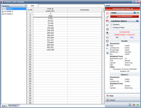
The next figure shows the generated failure times data. In this folio, the Advanced Systems View is used, so the data sheet shows the times-to-failure for system 2.
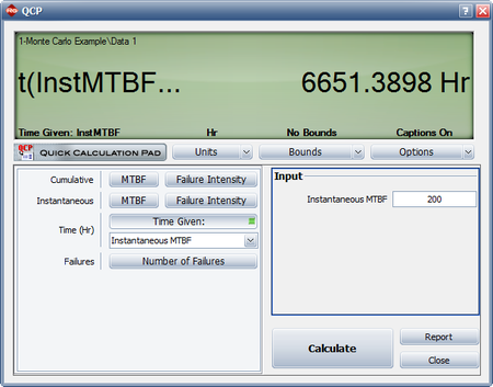
The data can then be analyzed just like a regular folio in the RGA software. In this case, we are interested in analyzing the data with the Crow-AMSAA (NHPP) model to calculate the demonstrated MTBF at the end of the test. In the Results area of the folio (shown in the figure above), it can be seen that the demonstrated MTBF at the end of the test is 189.83 hours. Since that does not meet the requirement of demonstrating an MTBF of 200 hours, we can either generate a new Monte Carlo data set with different time termination settings, or access the Quick Calculation Pad (QCP) in this folio to find the time for which the demonstrated (instantaneous) MTBF becomes 200 hours, as shown in the following figure. From the QCP it can be seen that, based on this specific data set, 6651.38 total operating hours are needed to show a demonstrated MTBF of 200 hours.
Note that since the Monte Carlo routine generates random input variables that follow the NHPP based on the specific [math]\displaystyle{ \beta \,\! }[/math] and [math]\displaystyle{ \lambda \,\! }[/math] values, if the same seed is not used the failure times will be different the next time you run the Monte Carlo routine. Also, because the input variables are pulled from an NHPP with the expected values of [math]\displaystyle{ \beta \,\! }[/math] and [math]\displaystyle{ \lambda ,\,\! }[/math] it should not be expected that the calculated parameters of the generated data set will match exactly the input parameters that were specified. In this example, the input parameters were set as [math]\displaystyle{ \beta =0.5\,\! }[/math] and [math]\displaystyle{ \lambda =0.75\,\! }[/math], and the data set based on the Monte Carlo generated failure times yielded Crow-AMSAA (NHPP) parameters of [math]\displaystyle{ \beta =0.4939\,\! }[/math] and [math]\displaystyle{ \lambda =0.8716\,\! }[/math]. The next time a data set is generated with a random seed, the calculated parameters will be slightly different, since we are essentially pulling input variables from a predefined distribution. The more simulations that are run, the more the calculated parameters will converge with the expected parameters. In the RGA software, the total number of generated failures with the Monte Carlo utility has to be less than 64,000.
SimuMatic
Reliability growth analysis using simulation can be a valuable tool for reliability practitioners. With this approach, reliability growth analyses are performed a large number of times on data sets that have been created using Monte Carlo simulation.
The RGA software's SimuMatic utility generates calculated values of beta and lambda parameters, based on user specified input parameters of beta and lambda. SimuMatic essentially performs a number of Monte Carlo simulations based on user-defined required test time or failure termination settings, and then recalculates the beta and lambda parameters for each of the generated data sets. The number of times that the Monte Carlo data sets are generated and the parameters are re-calculated is also user defined. The final output presents the calculated values of beta and lambda, and allows for various types of analysis.
To access the SimuMatic utility, choose Insert > Tools > Add SimuMatic. For all of the data sets, the basic parameters that are always specified are the beta [math]\displaystyle{ (\beta )\,\! }[/math] and lambda [math]\displaystyle{ (\lambda )\,\! }[/math] parameters of the Crow-AMSAA (NHPP) model or the power law model.
- Failure Times: The data set is generated assuming a single system. There is a choice between a time terminated test, where the termination time needs to be specified, or a failure terminated test, where the number of failures needs to be specified. SimuMatic will return the calculated values of [math]\displaystyle{ \beta \,\! }[/math] and [math]\displaystyle{ \lambda \,\! }[/math] for a specified number of data sets.
- Grouped Failure Times: The data set is generated assuming a single system. There is a choice between a time terminated test, where the termination time needs to be specified, or a failure terminated test, where the number of failures needs to be specified. In addition, constant or user-defined intervals need to be specified for the grouping of the data. SimuMatic will return the calculated values of [math]\displaystyle{ \beta \,\! }[/math] and [math]\displaystyle{ \lambda \,\! }[/math] for a specified number of data sets.
- Multiple Systems - Concurrent: In this case, the number of systems needs to be specified. There is a choice between a time terminated test, where the termination time needs to be specified, or a failure terminated test, where the number of failures needs to be specified. SimuMatic will return the calculated values of [math]\displaystyle{ \beta \,\! }[/math] and [math]\displaystyle{ \lambda \,\! }[/math] for a specified number of data sets.
- Repairable Systems: In this case, the number of systems needs to be specified. There is a choice between a time terminated test, where the termination time needs to be specified, or a failure terminated test, where the number of failures needs to be specified. SimuMatic will return the calculated values of [math]\displaystyle{ \beta \,\! }[/math] and [math]\displaystyle{ \lambda \,\! }[/math] for a specified number of data sets.
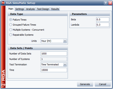
The next figure shows the Main tab of the SimuMatic window where all the necessary user inputs for a multiple systems - concurrent data set have been entered. The Analysis tab allows you to specify the confidence level for simulation-generated confidence bounds, while the Results tab gives you the option to compute for additional results, such as the instantaneous MTBF given a specific test time.
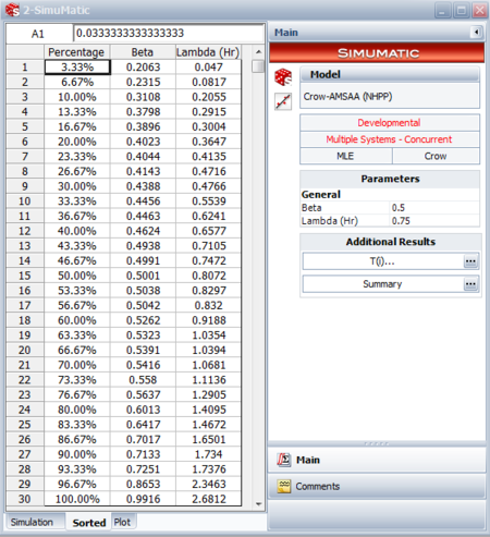
The next figure shows the generated results based on the inputs shown above. The data sheet called "Sorted" allows us to extract conclusions about the simulation-generated confidence bounds because the lambda and beta parameters and any other additional output are sorted by percentage.
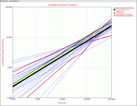
The following plot shows the simulation-confidence bounds for the cumulative number of failures based on the input parameters specified.
SimuMatic Example
A manufacturer wants to design a reliability growth test for a redesigned product, in order to achieve an MTBF of 1,000 hours. Simulation is chosen to estimate the 1-sided 90% confidence bound on the required time to achieve the goal MTBF of 1,000 hours and the 1-sided 90% lower confidence bound on the MTBF at the end of the test time. The total test time is expected to be 15,000 hours. Based on historical data for the previous version, the expected beta and lambda parameters of the test are 0.5 and 0.3, respectively. Do the following:
- 1) Generate 1,000 data sets using SimuMatic along with the required output.
- 2) Plot the instantaneous MTBF vs. time with the 90% confidence bounds.
- 3) Estimate the 1-sided 90% lower confidence bound on time for an MTBF of 1,000 hours.
- 4) Estimate the 1-sided 90% lower confidence bound on the instantaneous MTBF at the end of the test.
Solution
1) The next figure shows the SimuMatic window with all the appropriate inputs for creating the data sets.
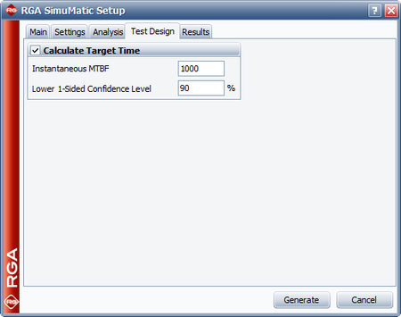
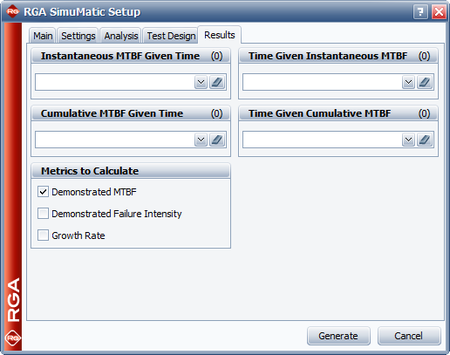
- The next two figures show the settings in the Analysis and Results tab of the SimuMatic window in order to obtain the desired outputs.
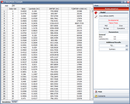
- The following figure displays the results of the simulation. The columns labeled "Beta" and "Lambda" contain the different parameters obtained by calculating each data set generated via simulation for the 1,000 data sets. The "IMTBF(15,000)" column contains the instantaneous MTBF at 15,000 hours (the end of test time), given the parameters obtained by calculating each data set generated via simulation. The "Target DMTBF" column contains the time required for the MTBF to reach 1,000 hours, given the parameters obtained from the simulation.
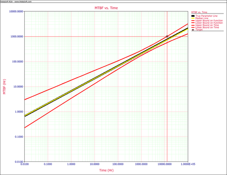
2) The next figure shows the plot of the instantaneous MTBF with the 90% confidence bounds.
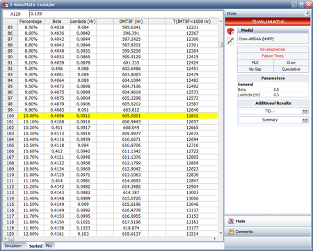
3) The 1-sided 90% lower confidence bound on time, assuming MTBF = 1,000 hours, can be obtained from the results of the simulation. In the "Sorted" data sheet, this is the target DMTBF value that corresponds to 10.00%, as shown in the next figure. Therefore the 1-sided 90% lower confidence bound on time is 12,642.21 hours.
4) The next figure shows the 1-sided 90% lower confidence bound on time in the instantaneous MTBF plot. This is indicated by the target lines on the plot.
5) The 1-sided 90% lower confidence bound on the instantaneous MTBF at the end of the test is again obtained from the "Sorted" data sheet by looking at the value in the "IMTBF(15,000)" column that corresponds to 10.00%. As seen in the simulation results shown above, the 1-sided 90% lower confidence bound on the instantaneous MTBF at the end of the test is 605.93 hours.

