Statistical Background on DOE

Variations occur in nature, be it the tensile strength of a particular grade of steel, caffeine content in your energy drink or the distance traveled by your vehicle in a day. Variations are also seen in the observations recorded during multiple executions of a process, even when all factors are strictly maintained at their respective levels and all the executions are run as identically as possible. The natural variations that occur in a process, even when all conditions are maintained at the same level, are often called noise. When the effect of a particular factor on a process is studied, it becomes extremely important to distinguish the changes in the process caused by the factor from noise. A number of statistical methods are available to achieve this. This chapter covers basic statistical concepts that are useful in understanding the statistical analysis of data obtained from designed experiments. The initial sections of this chapter discuss the normal distribution and related concepts. The assumption of the normal distribution is widely used in the analysis of designed experiments. The subsequent sections introduce the standard normal, chi-squared, [math]\displaystyle{ {t}\,\! }[/math] and [math]\displaystyle{ {F}\,\! }[/math] distributions that are widely used in calculations related to hypothesis testing and confidence bounds. The final sections of this chapter cover hypothesis testing. It is important to gain a clear understanding of hypothesis testing because this concept finds direct application in the analysis of designed experiments to determine whether or not a particular factor is significant [29].

Basic Concepts

Random Variables and the Normal Distribution

If you record the distance traveled by your car everyday, you'll notice that these values show some variation because your car does not travel the exact same distance every day. If a variable [math]\displaystyle{ {X}\,\! }[/math] is used to denote these values then [math]\displaystyle{ {X}\,\! }[/math] is termed as a random variable (because of the diverse and unpredicted values [math]\displaystyle{ {X}\,\! }[/math] can have). Random variables are denoted by uppercase letters while a measured value of the random variable is denoted by the corresponding lowercase letter. For example, if the distance traveled by your car on January 1 was 10.7 miles, then:

[math]\displaystyle{ x=10.7\text{ miles}\,\! }[/math]

A commonly used distribution to describe the behavior of random variables is the normal distribution. When you calculate the mean and standard deviation for a given data set, you are assuming that the data follows a normal distribution. A normal distribution (also referred to as the Gaussian distribution) is a bell-shaped curved (see figure below). The mean and standard deviation are the two parameters of this distribution. The mean determines the location of the distribution on the x-axis and is also called the location parameter of the normal distribution. The standard deviation determines the spread of the distribution (how narrow or wide) and is thus called the scale parameter of the normal distribution. The standard deviation, or its square called variance, gives an indication of the variability or spread of data. A large value of the standard deviation (or variance) implies that a large amount of variability exists in the data.

File:Doe3.1.png

Normal probability density functions for different values of mean and standard deviation.

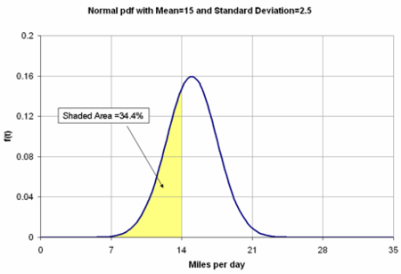
Any curve in the image below is also referred to as the probability density function or pdf of the normal distribution as the area under the curve gives the probability of occurrence of [math]\displaystyle{ X\,\! }[/math] for a particular interval. For instance, if you obtained the mean and standard deviation for the distance data of your car as 15 miles and 2.5 miles respectively, then the probability that your car travels a distance between 7 miles and 14 miles is given by the area under the curve covered between these two values, which is calculated to be 34.4% (see figure below). This means that on 34.4 days out of every 100 days your car travels, your car can be expected to cover a distance in the range of 7 to 14 miles.

Normal probability density function with the shaded area representing the probability of occurrence of data between 7 and 14 miles.

On a normal probability density function, the area under the curve between the values of [math]\displaystyle{ Mean-(3\times Standard Deviation)\,\! }[/math] and [math]\displaystyle{ Mean+(3\times Standard Deviation)\,\! }[/math] is approximately 99.7% of the total area under the curve. This implies that almost all the time (or 99.7% of the time) the distance traveled will fall in the range of 7.5 miles [math]\displaystyle{ (15-3\times 2.5)\,\! }[/math] and 22.5 miles [math]\displaystyle{ (15+3\times 2.5)\,\! }[/math]. Similarly, [math]\displaystyle{ Mean\pm (2\times Standard Deviation)\,\! }[/math] covers approximately 95% of the area under the curve and [math]\displaystyle{ Mean\pm (Standard Deviation)\,\! }[/math] covers approximately 68% of the area under the curve.

Population Mean, Sample Mean and Variance

If data for all of the population under investigation is known, then the mean and variance for this population can be calculated as follows:

Population Mean:

[math]\displaystyle{ \mu =\frac{\underset{i=1}{\overset{N}{\mathop{\sum }}}\,{{x}_{i}}}{N}\,\! }[/math]

Population Variance:

[math]\displaystyle{ {{\sigma }^{2}}=\frac{\underset{i=1}{\overset{N}{\mathop{\sum }}}\,{{({{x}_{i}}-\mu )}^{2}}}{N}\,\! }[/math]

Here, [math]\displaystyle{ N\,\! }[/math] is the size of the population.

The population standard deviation is the positive square root of the population variance.

Most of the time it is not possible to obtain data for the entire population. For example, it is impossible to measure the height of every male in a country to determine the average height and variance for males of a particular country. In such cases, results for the population have to be estimated using samples. This process is known as statistical inference. Mean and variance for a sample are calculated using the following relations:

Sample Mean:

[math]\displaystyle{ \bar{x}=\frac{\underset{i=1}{\overset{n}{\mathop{\sum }}}\,{{x}_{i}}}{n}\,\! }[/math]

Sample Variance:

[math]\displaystyle{ {{s}^{2}}=\frac{\underset{i=1}{\overset{n}{\mathop{\sum }}}\,{{({{x}_{i}}-\bar{x})}^{2}}}{n-1}\,\! }[/math]

Here, [math]\displaystyle{ n\,\! }[/math] is the sample size. The sample standard deviation is the positive square root of the sample variance. The sample mean and variance of a random sample can be used as estimators of the population mean and variance, respectively. The sample mean and variance are referred to as statistics. A statistic is any function of observations in a random sample. You may have noticed that the denominator in the calculation of sample variance, unlike the denominator in the calculation of population variance, is [math]\displaystyle{ (n-1)\,\! }[/math] and not [math]\displaystyle{ n\,\! }[/math]. The reason for this difference is explained in Biased Estimators.

Central Limit Theorem

The Central Limit Theorem states that for a large sample size, [math]\displaystyle{ n\,\! }[/math]:

• The sample means from a population are normally distributed with a mean value equal to the population mean, [math]\displaystyle{ \mu\,\! }[/math], even if the population is not normally distributed.

What this means is that if random samples are drawn from any population and the sample mean, [math]\displaystyle{ \bar{x}\,\! }[/math], calculated for each of these samples, then these sample means would follow the normal distribution with a mean (or location parameter) equal to the population mean, [math]\displaystyle{ \mu\,\! }[/math]. Thus, the distribution of the statistic, [math]\displaystyle{ \bar{x}\,\! }[/math], would be a normal distribution with mean, [math]\displaystyle{ \mu\,\! }[/math]. The distribution of a statistic is called the sampling distribution.

• The variance, [math]\displaystyle{ {{s}^{2}}\,\! }[/math], of the sample means would be [math]\displaystyle{ n\,\! }[/math] times smaller than the variance of the population, [math]\displaystyle{ {{\sigma }^{2}}\,\! }[/math].

This implies that the sampling distribution of the sample means would have a variance equal to [math]\displaystyle{ {{\sigma }^{2}}/n\,\! }[/math] (or a scale parameter equal to [math]\displaystyle{ \sigma /\sqrt{n}\,\! }[/math]), where [math]\displaystyle{ \sigma\,\! }[/math] is the population standard deviation. The standard deviation of the sampling distribution of an estimator is called the standard error of the estimator. Thus the standard error of sample mean [math]\displaystyle{ \bar{x}\,\! }[/math] is [math]\displaystyle{ \sigma /\sqrt{n}\,\! }[/math].

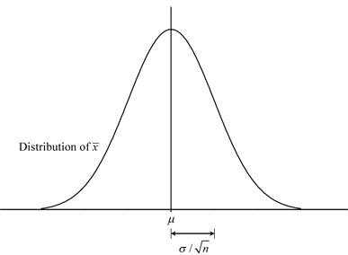
In short, the Central Limit Theorem states that the sampling distribution of the sample mean is a normal distribution with parameters [math]\displaystyle{ \mu\,\! }[/math] and [math]\displaystyle{ \sigma /\sqrt{n}\,\! }[/math] as shown in the figure below.

Sampling distribution of the sample mean. The distribution is normal with the mean equal to the population mean and the variance equal to the nth fraction of the population variance.

Unbiased and Biased Estimators

If the mean value of an estimator equals the true value of the quantity it estimates, then the estimator is called an unbiased estimator (see figure below). For example, assume that the sample mean is being used to estimate the mean of a population. Using the Central Limit Theorem, the mean value of the sample mean equals the population mean. Therefore, the sample mean is an unbiased estimator of the population mean. If the mean value of an estimator is either less than or greater than the true value of the quantity it estimates, then the estimator is called a biased estimator. For example, suppose you decide to choose the smallest observation in a sample to be the estimator of the population mean. Such an estimator would be biased because the average of the values of this estimator would always be less than the true population mean. In other words, the mean of the sampling distribution of this estimator would be less than the true value of the population mean it is trying to estimate. Consequently, the estimator is a biased estimator.

Example showing the distribution of a biased estimator which underestimated the parameter in question, along with the distribution of an unbiased estimator.

A case of biased estimation is seen to occur when sample variance, [math]\displaystyle{ {{s}^{2}}\,\! }[/math], is used to estimate the population variance, [math]\displaystyle{ {{\sigma }^{2}}\,\! }[/math], if the following relation is used to calculate the sample variance:

[math]\displaystyle{ {{s}^{2}}=\frac{\underset{i=1}{\overset{n}{\mathop{\sum }}}\,{{({{x}_{i}}-\bar{x})}^{2}}}{n}\,\! }[/math]

The sample variance calculated using this relation is always less than the true population variance. This is because deviations with respect to the sample mean, [math]\displaystyle{ \bar{x}\,\! }[/math], are used to calculate the sample variance. Sample observations, [math]\displaystyle{ {{x}_{i}}\,\! }[/math], tend to be closer to [math]\displaystyle{ \bar{x}\,\! }[/math] than to [math]\displaystyle{ \mu\,\! }[/math]. Thus, the calculated deviations [math]\displaystyle{ ({{x}_{i}}-\bar{x})\,\! }[/math] are smaller. As a result, the sample variance obtained is smaller than the population variance. To compensate for this, [math]\displaystyle{ (n-1)\,\! }[/math] is used as the denominator in place of [math]\displaystyle{ n\,\! }[/math] in the calculation of sample variance. Thus, the correct formula to obtain the sample variance is:

[math]\displaystyle{ {{s}^{2}}=\frac{\underset{i=1}{\overset{n}{\mathop{\sum }}}\,{{({{x}_{i}}-\bar{x})}^{2}}}{n-1}\,\! }[/math]

It is important to note that although using [math]\displaystyle{ (n-1)\,\! }[/math] as the denominator makes the sample variance, [math]\displaystyle{ {{s}^{2}}\,\! }[/math], an unbiased estimator of the population variance, [math]\displaystyle{ {{\sigma }^{2}}\,\! }[/math], the sample standard deviation, [math]\displaystyle{ s\,\! }[/math], still remains a biased estimator of the population standard deviation, [math]\displaystyle{ \sigma\,\! }[/math]. For large sample sizes this bias is negligible.

Degrees of Freedom (dof)

The number of degrees of freedom is the number of independent observations made in excess of the unknowns. If there are 3 unknowns and 7 independent observations are taken, then the number of degrees of freedom is 4 (7-3). As another example, two parameters are needed to specify a line. Therefore, there are 2 unknowns. If 10 points are available to fit the line, the number of degrees of freedom is 8 (10-2).

Standard Normal Distribution

A normal distribution with mean [math]\displaystyle{ \mu =0\,\! }[/math] and variance [math]\displaystyle{ {{\sigma }^{2}}=1\,\! }[/math] is called the standard normal distribution (see figure below). Standard normal random variables are denoted by [math]\displaystyle{ Z\,\!\,\! }[/math]. If [math]\displaystyle{ X\,\! }[/math] represents a normal random variable that follows the normal distribution with mean [math]\displaystyle{ \mu\,\! }[/math] and variance [math]\displaystyle{ {{\sigma }^{2}}\,\! }[/math], then the corresponding standard normal random variable is:

[math]\displaystyle{ Z=(X-\mu )/\sigma\,\! }[/math]

[math]\displaystyle{ Z\,\! }[/math] represents the distance of [math]\displaystyle{ X\,\! }[/math] from the mean [math]\displaystyle{ \mu\,\! }[/math] in terms of the standard deviation [math]\displaystyle{ \sigma\,\! }[/math].

Standard normal distribution.

Chi-Squared Distribution

If [math]\displaystyle{ Z\,\! }[/math] is a standard normal random variable, then the distribution of [math]\displaystyle{ {{Z}^{2}}\,\! }[/math] is a chi-squared distribution (see figure below).

Chi-squared distribution.

A chi-squared random variable is represented by [math]\displaystyle{ {{\chi }^{2}}\,\! }[/math]. Thus:

[math]\displaystyle{ {{\chi }^{2}}={{Z}^{2}}\,\! }[/math]

The distribution of the variable [math]\displaystyle{ {{\chi }^{2}}\,\! }[/math] mentioned in the previous equation is also referred to as centrally distributed chi-squared with one degree of freedom. The degree of freedom is 1 here because the chi-squared random variable is obtained from a single standard normal random variable [math]\displaystyle{ Z\,\! }[/math]. The previous equation may also be represented by including the degree of freedom in the equation as:

[math]\displaystyle{ \chi _{1}^{2}={{Z}^{2}}\,\! }[/math]

If [math]\displaystyle{ {{Z}_{1}}\,\! }[/math], [math]\displaystyle{ {{Z}_{2}}\,\! }[/math], [math]\displaystyle{ {{Z}_{3}}\,\! }[/math]... [math]\displaystyle{ {{Z}_{m}}\,\! }[/math] are [math]\displaystyle{ m\,\! }[/math] independent standard normal random variables, then:

[math]\displaystyle{ \chi _{m}^{2}=Z_{1}^{2}+Z_{2}^{2}+Z_{3}^{2}...+Z_{m}^{2}\,\! }[/math]

is also a chi-squared random variable. The distribution of [math]\displaystyle{ \chi _{m}^{2}\,\! }[/math] is said to be centrally distributed chi-squared with [math]\displaystyle{ m\,\! }[/math] degrees of freedom, as the chi-squared random variable is obtained from [math]\displaystyle{ m\,\! }[/math] independent standard normal random variables. If [math]\displaystyle{ X\,\! }[/math] is a normal random variable, then the distribution of [math]\displaystyle{ {{X}^{2}}\,\! }[/math] is said to be non-centrally distributed chi-squared with one degree of freedom. Therefore, [math]\displaystyle{ {{X}^{2}}\,\! }[/math] is a chi-squared random variable and can be represented as:

[math]\displaystyle{ \chi _{1}^{2}={{X}^{2}}\,\! }[/math]

If [math]\displaystyle{ {{X}_{1}}\,\! }[/math], [math]\displaystyle{ {{X}_{2}}\,\! }[/math], [math]\displaystyle{ {{X}_{3}}\,\! }[/math]... [math]\displaystyle{ {{X}_{m}}\,\! }[/math] are [math]\displaystyle{ m\,\! }[/math] independent normal random variables then:

[math]\displaystyle{ \chi _{m}^{2}=X_{1}^{2}+X_{2}^{2}+X_{3}^{2}...+X_{m}^{2}\,\! }[/math]

is a non-centrally distributed chi-squared random variable with [math]\displaystyle{ m\,\! }[/math] degrees of freedom.

Student's t Distribution (t Distribution)

If [math]\displaystyle{ Z\,\! }[/math] is a standard normal random variable, [math]\displaystyle{ \chi _{k}^{2}\,\! }[/math] is a chi-squared random variable with [math]\displaystyle{ k\,\! }[/math] degrees of freedom, and both of these random variables are independent, then the distribution of the random variable [math]\displaystyle{ T\,\! }[/math] such that:

[math]\displaystyle{ T=\frac{Z}{\sqrt{\chi _{k}^{2}/k}}\,\! }[/math]

is said to follow the [math]\displaystyle{ t\,\! }[/math] distribution with [math]\displaystyle{ k\,\! }[/math] degrees of freedom.

The [math]\displaystyle{ t\,\! }[/math] distribution is similar in appearance to the standard normal distribution (see figure below). Both of these distributions are symmetric, reaching a maximum at the mean value of zero. However, the [math]\displaystyle{ t\,\! }[/math] distribution has heavier tails than the standard normal distribution, implying that it has more probability in the tails. As the degrees of freedom, [math]\displaystyle{ k\,\! }[/math], of the [math]\displaystyle{ t\,\! }[/math] distribution approach infinity, the distribution approaches the standard normal distribution.

[math]\displaystyle{ t\,\! }[/math] distribution.

F Distribution

If [math]\displaystyle{ \chi _{u}^{2}\,\! }[/math] and [math]\displaystyle{ \chi _{v}^{2}\,\! }[/math] are two independent chi-squared random variables with [math]\displaystyle{ u\,\! }[/math] and [math]\displaystyle{ v\,\! }[/math] degrees of freedom, respectively, then the distribution of the random variable [math]\displaystyle{ F\,\! }[/math] such that:

[math]\displaystyle{ F=\frac{\chi _{u}^{2}/u}{\chi _{v}^{2}/v}\,\! }[/math]

is said to follow the [math]\displaystyle{ F\,\! }[/math] distribution with [math]\displaystyle{ u\,\! }[/math] degrees of freedom in the numerator and [math]\displaystyle{ v\,\! }[/math] degrees of freedom in the denominator. The [math]\displaystyle{ F\,\! }[/math] distribution resembles the chi-squared distribution (see the following figure). This is because the [math]\displaystyle{ F\,\! }[/math] random variable, like the chi-squared random variable, is non-negative and the distribution is skewed to the right (a right skew means that the distribution is unsymmetrical and has a right tail). The [math]\displaystyle{ F\,\! }[/math] random variable is usually abbreviated by including the degrees of freedom as [math]\displaystyle{ {{F}_{u,v}}\,\! }[/math].

[math]\displaystyle{ F\,\! }[/math] distribution.

Hypothesis Testing

A statistical hypothesis is a statement about the population under study or about the distribution of a quantity under consideration. The null hypothesis, [math]\displaystyle{ {{H}_{0}}\,\! }[/math], is the hypothesis to be tested. It is a statement about a theory that is believed to be true but has not been proven. For instance, if a new product design is thought to perform consistently, regardless of the region of operation, then the null hypothesis may be stated as

[math]\displaystyle{ {{H}_{0}}\text{ : New product design performance is not affected by region}\,\! }[/math]

Statements in [math]\displaystyle{ {{H}_{0}}\,\! }[/math] always include exact values of parameters under consideration. For example:

[math]\displaystyle{ {{H}_{0}}\text{ : The population mean is 100}\,\! }[/math]

Or simply:

[math]\displaystyle{ {{H}_{0}}:\mu =100\,\! }[/math]

Rejection of the null hypothesis, [math]\displaystyle{ {{H}_{0}}\,\! }[/math], leads to the possibility that the alternative hypothesis, [math]\displaystyle{ {{H}_{1}}\,\! }[/math], may be true. Given the previous null hypothesis, the alternate hypothesis may be:

[math]\displaystyle{ {{H}_{1}}\text{ : New product design performance is affected by region}\,\! }[/math]

In the case of the example regarding inference on the population mean, the alternative hypothesis may be stated as:

[math]\displaystyle{ {{H}_{1}}\text{ : The population mean is not 100}\,\! }[/math]

Or simply:

[math]\displaystyle{ {{H}_{1}}:\mu \ne 100\,\! }[/math]

Hypothesis testing involves the calculation of a test statistic based on a random sample drawn from the population. The test statistic is then compared to the critical value(s) and used to make a decision about the null hypothesis. The critical values are set by the analyst.

The outcome of a hypothesis test is that we either reject [math]\displaystyle{ {{H}_{0}}\,\! }[/math] or we fail to reject [math]\displaystyle{ {{H}_{0}}\,\! }[/math]. Failing to reject [math]\displaystyle{ {{H}_{0}}\,\! }[/math] implies that we did not find sufficient evidence to reject [math]\displaystyle{ {{H}_{0}}\,\! }[/math]. It does not necessarily mean that there is a high probability that [math]\displaystyle{ {{H}_{0}}\,\! }[/math] is true. As such, the terminology accept [math]\displaystyle{ {{H}_{0}}\,\! }[/math] is not preferred.

For example, assume that an analyst wants to know if the mean of a certain population is 100 or not. The statements for this hypothesis can be stated as follows:

[math]\displaystyle{ \begin{align} & {{H}_{0}}: & \mu =100 \\ & {{H}_{1}}: & \mu \ne 100 \end{align}\,\! }[/math]

The analyst decides to use the sample mean as the test statistic for this test. The analyst further decides that if the sample mean lies between 98 and 102 it can be concluded that the population mean is 100. Thus, the critical values set for this test by the analyst are 98 and 102. It is also decided to draw out a random sample of size 25 from the population.

Now assume that the true population mean is [math]\displaystyle{ \mu =100\,\! }[/math] and the true population standard deviation is [math]\displaystyle{ \sigma =5\,\! }[/math]. This information is not known to the analyst. Using the Central Limit Theorem, the test statistic (sample mean) will follow a normal distribution with a mean equal to the population mean, [math]\displaystyle{ \mu\,\! }[/math], and a standard deviation of [math]\displaystyle{ \sigma /\sqrt{n}\,\! }[/math], where [math]\displaystyle{ n\,\! }[/math] is the sample size. Therefore, the distribution of the test statistic has a mean of 100 and a standard deviation of [math]\displaystyle{ 5/\sqrt{25}=1\,\! }[/math]. This distribution is shown in the figure below.

The unshaded area in the figure bound by the critical values of 98 and 102 is called the acceptance region. The acceptance region gives the probability that a random sample drawn from the population would have a sample mean that lies between 98 and 102. Therefore, this is the region that will lead to the "acceptance" of [math]\displaystyle{ {{H}_{0}}\,\! }[/math]. On the other hand, the shaded area gives the probability that the sample mean obtained from the random sample lies outside of the critical values. In other words, it gives the probability of rejection of the null hypothesis when the true mean is 100. The shaded area is referred to as the critical region or the rejection region. Rejection of the null hypothesis [math]\displaystyle{ {{H}_{0}}\,\! }[/math] when it is true is referred to as type I error. Thus, there is a 4.56% chance of making a type I error in this hypothesis test. This percentage is called the significance level of the test and is denoted by [math]\displaystyle{ \alpha\,\! }[/math]. Here [math]\displaystyle{ \alpha =0.0456\,\! }[/math] or [math]\displaystyle{ 4.56%\,\! }[/math] (area of the shaded region in the figure). The value of [math]\displaystyle{ \alpha\,\! }[/math] is set by the analyst when he/she chooses the critical values.

Acceptance region and critical regions for the hypothesis test.

A type II error is also defined in hypothesis testing. This error occurs when the analyst fails to reject the null hypothesis when it is actually false. Such an error would occur if the value of the sample mean obtained is in the acceptance region bounded by 98 and 102 even though the true population mean is not 100. The probability of occurrence of type II error is denoted by [math]\displaystyle{ \beta\,\! }[/math].

Two-sided and One-sided Hypotheses

As seen in the previous section, the critical region for the hypothesis test is split into two parts, with equal areas in each tail of the distribution of the test statistic. Such a hypothesis, in which the values for which we can reject [math]\displaystyle{ {{H}_{0}}\,\! }[/math] are in both tails of the probability distribution, is called a two-sided hypothesis. The hypothesis for which the critical region lies only in one tail of the probability distribution is called a one-sided hypothesis. For instance, consider the following hypothesis test:

[math]\displaystyle{ \begin{align} & {{H}_{0}}: & \mu =100 \\ & {{H}_{1}}: & \mu \gt 100 \end{align}\,\! }[/math]

This is an example of a one-sided hypothesis. Here the critical region lies entirely in the right tail of the distribution.

The hypothesis test may also be set up as follows:

[math]\displaystyle{ \begin{align} & {{H}_{0}}: & \mu =100 \\ & {{H}_{1}}: & \mu \lt 100 \end{align}\,\! }[/math]

This is also a one-sided hypothesis. Here the critical region lies entirely in the left tail of the distribution.

Statistical Inference for a Single Sample

Hypothesis testing forms an important part of statistical inference. As stated previously, statistical inference refers to the process of estimating results for the population based on measurements from a sample. In the next sections, statistical inference for a single sample is discussed briefly.

Inference on the Mean of a Population When the Variance Is Known

The test statistic used in this case is based on the standard normal distribution. If [math]\displaystyle{ \bar{X}\,\! }[/math] is the calculated sample mean, then the standard normal test statistic is:

[math]\displaystyle{ {{Z}_{0}}=\frac{\bar{X}-{{\mu }_{0}}}{\sigma /\sqrt{n}}\,\! }[/math]

where [math]\displaystyle{ {{\mu }_{0}}\,\! }[/math] is the hypothesized population mean, [math]\displaystyle{ \sigma\,\! }[/math] is the population standard deviation and [math]\displaystyle{ n\,\! }[/math] is the sample size.

One-sided hypothesis where the critical region lies in the right tail.

One-sided hypothesis where the critical region lies in the left tail.

For example, assume that an analyst wants to know if the mean of a population, [math]\displaystyle{ \mu\,\! }[/math], is 100. The population variance, [math]\displaystyle{ {{\sigma }^{2}}\,\! }[/math], is known to be 25. The hypothesis test may be conducted as follows:

1) The statements for this hypothesis test may be formulated as:

[math]\displaystyle{ \begin{align} & {{H}_{0}}: & \mu =100 \\ & {{H}_{1}}: & \mu \ne 100 \end{align}\,\! }[/math]

It is a clear that this is a two-sided hypothesis. Thus the critical region will lie in both of the tails of the probability distribution.

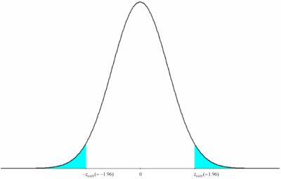
2) Assume that the analyst chooses a significance level of 0.05. Thus [math]\displaystyle{ \alpha =0.05\,\! }[/math]. The significance level determines the critical values of the test statistic. Here the test statistic is based on the standard normal distribution. For the two-sided hypothesis these values are obtained as:

[math]\displaystyle{ {{z}_{\alpha /2}}={{z}_{0.025}}=1.96\,\! }[/math]

and

[math]\displaystyle{ -{{z}_{\alpha /2}}=-{{z}_{0.025}}=-1.96\,\! }[/math]

These values and the critical regions are shown in figure below. The analyst would fail to reject [math]\displaystyle{ {{H}_{0}}\,\! }[/math] if the test statistic, [math]\displaystyle{ {{Z}_{0}}\,\! }[/math], is such that:

[math]\displaystyle{ -{{z}_{\alpha /2}}\le {{Z}_{0}}\le {{z}_{\alpha /2}}\,\! }[/math]

or

[math]\displaystyle{ -1.96\le {{Z}_{0}}\le 1.96\,\! }[/math]

3) Next the analyst draws a random sample from the population. Assume that the sample size, [math]\displaystyle{ n\,\! }[/math], is 25 and the sample mean is obtained as [math]\displaystyle{ \bar{x}=103\,\! }[/math].

Critical values and rejection region marked on the standard normal distribution.

4) The value of the test statistic corresponding to the sample mean value of 103 is:

[math]\displaystyle{ \begin{align} {{z}_{0}}&=& \frac{\bar{x}-{{\mu }_{0}}}{\sigma /\sqrt{n}} \\ &=& \frac{103-100}{5/\sqrt{25}} \\ &=& 3 \end{align}\,\! }[/math]

Since this value does not lie in the acceptance region [math]\displaystyle{ -1.96\le {{Z}_{0}}\le 1.96\,\! }[/math], we reject [math]\displaystyle{ {{H}_{0}}:\mu =100\,\! }[/math] at a significance level of 0.05.

P Value

In the previous example the null hypothesis was rejected at a significance level of 0.05. This statement does not provide information as to how far out the test statistic was into the critical region. At times it is necessary to know if the test statistic was just into the critical region or was far out into the region. This information can be provided by using the [math]\displaystyle{ p\,\! }[/math] value.

The [math]\displaystyle{ p\,\! }[/math] value is the probability of occurrence of the values of the test statistic that are either equal to the one obtained from the sample or more unfavorable to [math]\displaystyle{ {{H}_{0}}\,\! }[/math] than the one obtained from the sample. It is the lowest significance level that would lead to the rejection of the null hypothesis, [math]\displaystyle{ {{H}_{0}}\,\! }[/math], at the given value of the test statistic. The value of the test statistic is referred to as significant when [math]\displaystyle{ {{H}_{0}}\,\! }[/math] is rejected. The [math]\displaystyle{ p\,\! }[/math] value is the smallest [math]\displaystyle{ \alpha\,\! }[/math] at which the statistic is significant and [math]\displaystyle{ {{H}_{0}}\,\! }[/math] is rejected.

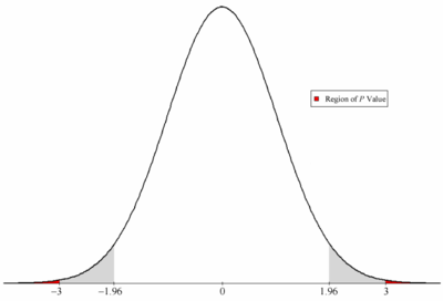
For instance, in the previous example the test statistic was obtained as [math]\displaystyle{ {{z}_{0}}=3\,\! }[/math]. Values that are more unfavorable to [math]\displaystyle{ {{H}_{0}}\,\! }[/math] in this case are values greater than 3. Then the required probability is the probability of getting a test statistic value either equal to or greater than 3 (this is abbreviated as [math]\displaystyle{ P(Z\ge 3)\,\! }[/math]). This probability is shown in figure below as the dark shaded area on the right tail of the distribution and is equal to 0.0013 or 0.13% (i.e., [math]\displaystyle{ P(Z\ge 3)=0.0013\,\! }[/math]). Since this is a two-sided test the [math]\displaystyle{ p\,\! }[/math] value is:

[math]\displaystyle{ p\text{ }value=2\times 0.0013=0.0026\,\! }[/math]

Therefore, the smallest [math]\displaystyle{ \alpha\,\! }[/math] (corresponding to the test static value of 3) that would lead to the rejection of [math]\displaystyle{ {{H}_{0}}\,\! }[/math] is 0.0026.

[math]\displaystyle{ P\,\! }[/math] value.

Inference on Mean of a Population When Variance Is Unknown

When the variance, [math]\displaystyle{ {{\sigma }^{2}}\,\! }[/math], of a population (that can be assumed to be normally distributed) is unknown the sample variance, [math]\displaystyle{ {{S}^{2}}\,\! }[/math], is used in its place in the calculation of the test statistic. The test statistic used in this case is based on the [math]\displaystyle{ t\,\! }[/math] distribution and is obtained using the following relation:

[math]\displaystyle{ {{T}_{0}}=\frac{\bar{X}-{{\mu }_{0}}}{S/\sqrt{n}}\,\! }[/math]

The test statistic follows the [math]\displaystyle{ t\,\! }[/math] distribution with [math]\displaystyle{ n-1\,\! }[/math] degrees of freedom.

For example, assume that an analyst wants to know if the mean of a population, [math]\displaystyle{ \mu\,\! }[/math], is less than 50 at a significance level of 0.05. A random sample drawn from the population gives the sample mean, [math]\displaystyle{ \bar{x}\,\! }[/math], as 47.7 and the sample standard deviation, [math]\displaystyle{ s\,\! }[/math], as 5. The sample size, [math]\displaystyle{ n\,\! }[/math], is 25. The hypothesis test may be conducted as follows:

1) The statements for this hypothesis test may be formulated as:

[math]\displaystyle{ \begin{align} & {{H}_{0}}: & \mu =50 \\ & {{H}_{1}}: & \mu \lt 50 \end{align}\,\! }[/math]

It is clear that this is a one-sided hypothesis. Here the critical region will lie in the left tail of the probability distribution.

2) Significance level, [math]\displaystyle{ \alpha =0.05\,\! }[/math]. Here, the test statistic is based on the [math]\displaystyle{ t\,\! }[/math] distribution. Thus, for the one-sided hypothesis the critical value is obtained as:

[math]\displaystyle{ -{{t}_{\alpha ,dof}}=-{{t}_{0.05,n-1}}=-{{t}_{0.05,24}}=-1.7109\,\! }[/math]

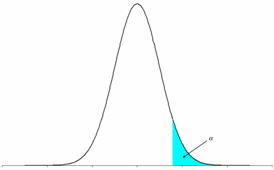
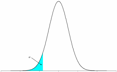
This value and the critical regions are shown in the figure below. The analyst would fail to reject [math]\displaystyle{ {{H}_{0}}\,\! }[/math] if the test statistic [math]\displaystyle{ {{T}_{0}}\,\! }[/math] is such that:

[math]\displaystyle{ {{T}_{0}}\gt -{{t}_{0.05,24}}\,\! }[/math]

3) The value of the test statistic, [math]\displaystyle{ {{T}_{0}}\,\! }[/math], corresponding to the given sample data is:

[math]\displaystyle{ \begin{align}{{t}_{0}}= & \frac{\bar{X}-{{\mu }_{0}}}{S/\sqrt{n}} \\ = & \frac{47.7-50}{5/\sqrt{25}} \\ = & -2.3 \end{align}\,\! }[/math]

Since [math]\displaystyle{ {{T}_{0}}\,\! }[/math] is less than the critical value of -1.7109, [math]\displaystyle{ {{H}_{0}}:\mu =50\,\! }[/math] is rejected and it is concluded that at a significance level of 0.05 the population mean is less than 50.

4) [math]\displaystyle{ P\,\! }[/math] value

In this case the [math]\displaystyle{ p\,\! }[/math] value is the probability that the test statistic is either less than or equal to [math]\displaystyle{ -2.3\,\! }[/math] (since values less than [math]\displaystyle{ -2.3\,\! }[/math] are unfavorable to [math]\displaystyle{ {{H}_{0}}\,\! }[/math]). This probability is equal to 0.0152.

Critical value and rejection region marked on the [math]\displaystyle{ t\,\! }[/math] distribution.

Inference on Variance of a Normal Population

The test statistic used in this case is based on the Chi-Squared distribution. If [math]\displaystyle{ {{S}^{2}}\,\! }[/math] is the calculated sample variance and [math]\displaystyle{ \sigma _{0}^{2}\,\! }[/math] the hypothesized population variance then the Chi-Squared test statistic is:

[math]\displaystyle{ \chi _{0}^{2}=\frac{(n-1){{S}^{2}}}{\sigma _{0}^{2}}\,\! }[/math]

The test statistic follows the Chi-Squared distribution with [math]\displaystyle{ n-1\,\! }[/math] degrees of freedom.

For example, assume that an analyst wants to know if the variance of a population exceeds 1 at a significance level of 0.05. A random sample drawn from the population gives the sample variance as 2. The sample size, [math]\displaystyle{ n\,\! }[/math], is 20. The hypothesis test may be conducted as follows:

1) The statements for this hypothesis test may be formulated as:

[math]\displaystyle{ \begin{align} & {{H}_{0}}: & {{\sigma }^{2}}=1 \\ & {{H}_{1}}: & {{\sigma }^{2}}\gt 1 \end{align}\,\! }[/math]

This is a one-sided hypothesis. Here the critical region will lie in the right tail of the probability distribution.

2) Significance level, [math]\displaystyle{ \alpha =0.05\,\! }[/math]. Here, the test statistic is based on the Chi-Squared distribution. Thus for the one-sided hypothesis the critical value is obtained as:

[math]\displaystyle{ \chi _{\alpha ,n-1}^{2}=\chi _{0.05,19}^{2}=30.1435\,\! }[/math]

This value and the critical regions are shown in the figure below. The analyst would fail to reject [math]\displaystyle{ {{H}_{0}}\,\! }[/math] if the test statistic [math]\displaystyle{ \chi _{0}^{2}\,\! }[/math] is such that:

[math]\displaystyle{ \chi _{0}^{2}\lt \chi _{0.05,19}^{2}\,\! }[/math]

3) The value of the test statistic [math]\displaystyle{ \chi _{0}^{2}\,\! }[/math] corresponding to the given sample data is:

[math]\displaystyle{ \begin{align} \chi _{0}^{2} &=&\frac{(n-1){{S}^{2}}}{\sigma _{0}^{2}} \\ & = & \frac{(20-1)2}{1}=38 \end{align}\,\! }[/math]

Since [math]\displaystyle{ \chi _{0}^{2}\,\! }[/math] is greater than the critical value of 30.1435, [math]\displaystyle{ {{H}_{0}}:{{\sigma }^{2}}=1\,\! }[/math] is rejected and it is concluded that at a significance level of 0.05 the population variance exceeds 1.

Critical value and rejection region marked on the chi-squared distribution.

4) [math]\displaystyle{ P\,\! }[/math] value

In this case the [math]\displaystyle{ p\,\! }[/math] value is the probability that the test statistic is greater than or equal to 38 (since values greater than 38 are unfavorable to [math]\displaystyle{ {{H}_{0}}\,\! }[/math]). This probability is determined to be 0.0059.

Statistical Inference for Two Samples

Inference on the Difference in Population Means When Variances Are Known

The test statistic used here is based on the standard normal distribution. Let [math]\displaystyle{ {{\mu }_{1}}\,\! }[/math] and [math]\displaystyle{ {{\mu }_{2}}\,\! }[/math] represent the means of two populations, and [math]\displaystyle{ \sigma _{1}^{2}\,\! }[/math] and [math]\displaystyle{ \sigma _{2}^{2}\,\! }[/math] their variances, respectively. Let [math]\displaystyle{ {{\Delta }_{0}}\,\! }[/math] be the hypothesized difference in the population means and [math]\displaystyle{ {{\bar{X}}_{1}}\,\! }[/math] and [math]\displaystyle{ {{\bar{X}}_{2}}\,\! }[/math] be the sample means obtained from two samples of sizes [math]\displaystyle{ {{n}_{1}}\,\! }[/math] and [math]\displaystyle{ {{n}_{2}}\,\! }[/math] drawn randomly from the two populations, respectively. The test statistic can be obtained as:

[math]\displaystyle{ {{Z}_{0}}=\frac{{{{\bar{X}}}_{1}}-{{{\bar{X}}}_{2}}-{{\Delta }_{0}}}{\sqrt{\frac{\sigma _{1}^{2}}{{{n}_{1}}}+\frac{\sigma _{2}^{2}}{{{n}_{2}}}}}\,\! }[/math]

The statements for the hypothesis test are:

[math]\displaystyle{ \begin{align} & {{H}_{0}}: & {{\mu }_{1}}-{{\mu }_{2}}={{\Delta }_{0}} \\ & {{H}_{1}}: & {{\mu }_{1}}-{{\mu }_{2}}\ne {{\Delta }_{0}} \end{align}\,\! }[/math]

If [math]\displaystyle{ {{\Delta }_{0}}=0\,\! }[/math], then the hypothesis will test for the equality of the two population means.

Inference on the Difference in Population Means When Variances Are Unknown

If the population variances can be assumed to be equal then the following test statistic based on the [math]\displaystyle{ t\,\! }[/math] distribution can be used. Let [math]\displaystyle{ {{\bar{X}}_{1}}\,\! }[/math], [math]\displaystyle{ {{\bar{X}}_{2}}\,\! }[/math], [math]\displaystyle{ S_{1}^{2}\,\! }[/math] and [math]\displaystyle{ S_{2}^{2}\,\! }[/math] be the sample means and variances obtained from randomly drawn samples of sizes [math]\displaystyle{ {{n}_{1}}\,\! }[/math] and [math]\displaystyle{ {{n}_{2}}\,\! }[/math] from the two populations, respectively. The weighted average, [math]\displaystyle{ S_{p}^{2}\,\! }[/math], of the two sample variances is:

[math]\displaystyle{ \begin{align}S_{p}^{2}=\frac{({{n}_{1}}-1)S_{1}^{2}+({{n}_{2}}-1)S_{2}^{2}}{{{n}_{1}}+{{n}_{2}}-2}\end{align}\,\! }[/math]

[math]\displaystyle{ S_{p}^{2}\,\! }[/math] has ( [math]\displaystyle{ {{n}_{1}}\,\! }[/math] + [math]\displaystyle{ {{n}_{2}}\,\! }[/math] -- 2) degrees of freedom. The test statistic can be calculated as:

[math]\displaystyle{ \begin{align}{{T}_{0}}=\frac{{{{\bar{X}}}_{1}}-{{{\bar{X}}}_{2}}-{{\Delta }_{0}}}{{{S}_{p}}\sqrt{\frac{1}{{{n}_{1}}}+\frac{1}{{{n}_{2}}}}}\end{align}\,\! }[/math]

[math]\displaystyle{ {{T}_{0}}\,\! }[/math] follows the [math]\displaystyle{ t\,\! }[/math] distribution with ([math]\displaystyle{ {{n}_{1}}\,\! }[/math] + [math]\displaystyle{ {{n}_{2}}\,\! }[/math] -- 2) degrees of freedom. This test is also referred to as the two-sample pooled [math]\displaystyle{ t\,\! }[/math] test. If the population variances cannot be assumed to be equal then the following test statistic is used:

[math]\displaystyle{ \begin{align}T_{0}^{*}=\frac{{{{\bar{X}}}_{1}}-{{{\bar{X}}}_{2}}-{{\Delta }_{0}}}{\sqrt{\frac{S_{1}^{2}}{{{n}_{1}}}+\frac{S_{2}^{2}}{{{n}_{2}}}}}\end{align}\,\! }[/math]

[math]\displaystyle{ T_{0}^{*}\,\! }[/math] follows the [math]\displaystyle{ t\,\! }[/math] distribution with [math]\displaystyle{ \upsilon\,\! }[/math] degrees of freedom. [math]\displaystyle{ \upsilon\,\! }[/math] is defined as follows:

[math]\displaystyle{ \begin{align}\upsilon =\frac{{{\left( \frac{S_{1}^{2}}{{{n}_{1}}}+\frac{S_{2}^{2}}{{{n}_{2}}} \right)}^{2}}}{\frac{{{\left( S_{1}^{2}/{{n}_{1}} \right)}^{2}}}{{{n}_{1}}+1}+\frac{{{\left( S_{2}^{2}/{{n}_{2}} \right)}^{2}}}{{{n}_{2}}+1}}-2\end{align}\,\! }[/math]

Inference on the Variances of Two Normal Populations

The test statistic used here is based on the [math]\displaystyle{ F\,\! }[/math] distribution. If [math]\displaystyle{ S_{1}^{2}\,\! }[/math] and [math]\displaystyle{ S_{2}^{2}\,\! }[/math] are the sample variances drawn randomly from the two populations and [math]\displaystyle{ {{n}_{1}}\,\! }[/math] and [math]\displaystyle{ {{n}_{2}}\,\! }[/math] are the two sample sizes, respectively, then the test statistic that can be used to test the equality of the population variances is:

[math]\displaystyle{ {{F}_{0}}=\frac{S_{1}^{2}}{S_{2}^{2}}\,\! }[/math]

The test statistic follows the [math]\displaystyle{ F\,\! }[/math] distribution with ([math]\displaystyle{ {{n}_{1}}\,\! }[/math] -- 1) degrees of freedom in the numerator and ([math]\displaystyle{ {{n}_{2}}\,\! }[/math] -- 1) degrees of freedom in the denominator.

For example, assume that an analyst wants to know if the variances of two normal populations are equal at a significance level of 0.05. Random samples drawn from the two populations give the sample standard deviations as 1.84 and 2, respectively. Both the sample sizes are 20. The hypothesis test may be conducted as follows:

1) The statements for this hypothesis test may be formulated as:

[math]\displaystyle{ \begin{align} & {{H}_{0}}: & \sigma _{1}^{2}=\sigma _{2}^{2} \\ & {{H}_{1}}: & \sigma _{1}^{2}\ne \sigma _{2}^{2} \end{align}\,\! }[/math]

It is clear that this is a two-sided hypothesis and the critical region will be located on both sides of the probability distribution.

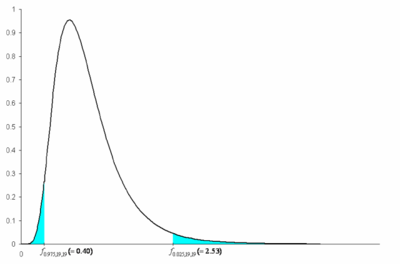
2) Significance level [math]\displaystyle{ \alpha =0.05\,\! }[/math]. Here the test statistic is based on the [math]\displaystyle{ F\,\! }[/math] distribution. For the two-sided hypothesis the critical values are obtained as:

[math]\displaystyle{ {{f}_{\alpha /2,{{n}_{1}}-1,{{n}_{2}}-1}}={{f}_{0.025,19,19}}=2.53\,\! }[/math]

and

[math]\displaystyle{ {{f}_{1-\alpha /2,{{n}_{1}}-1,{{n}_{2}}-1}}={{f}_{0.975,19,19}}=0.40\,\! }[/math]

These values and the critical regions are shown in the figure below. The analyst would fail to reject [math]\displaystyle{ {{H}_{0}}\,\! }[/math] if the test statistic [math]\displaystyle{ {{F}_{0}}\,\! }[/math] is such that:

[math]\displaystyle{ {{f}_{1-\alpha /2,{{n}_{1}}-1,{{n}_{2}}-1}}\le {{F}_{0}}\le {{f}_{\alpha /2,{{n}_{1}}-1,{{n}_{2}}-1}}\,\! }[/math]

or

[math]\displaystyle{ 0.40\le {{F}_{0}}\le 2.53\,\! }[/math]

3) The value of the test statistic [math]\displaystyle{ {{F}_{0}}\,\! }[/math] corresponding to the given data is:

[math]\displaystyle{ \begin{align} {{f}_{0}}= & \frac{S_{1}^{2}}{S_{2}^{2}} \\ = & \frac{{{1.84}^{2}}}{{{2}^{2}}} \\ = & 0.8464 \end{align}\,\! }[/math]

Since [math]\displaystyle{ {{F}_{0}}\,\! }[/math] lies in the acceptance region, the analyst fails to reject [math]\displaystyle{ {{H}_{0}}:\sigma _{1}^{2}=\sigma _{2}^{2}\,\! }[/math] at a significance level of 0.05.

Critical values and rejection region marked on the [math]\displaystyle{ F\,\! }[/math] distribution.