Reliability Test Design

This chapter discusses several methods for designing reliability tests. This includes:

• Reliability Demonstration Tests (RDT): Often used to demonstrate if the product reliability can meet the requirement. For this type of test design, four methods are supported in Weibull++:
  • Parametric Binomial: Used when the test duration is different from the time of the required reliability. An underlying distribution should be assumed.
  • Non-Parametric Binomial: No distribution assumption is needed for this test design method. It can be used for one shot devices.
  • Exponential Chi-Squared: Designed for exponential failure time.
  • Non-Parametric Bayesian: Integrated Bayesian theory with the traditional non-parametric binomial method.
• Expected Failure Times Plot: Can help the engineer determine the expected test duration when the total sample size is known and the allowed number of failures is given.
• Difference Detection Matrix: Can help the engineer design a test to compare the BX% life or mean life of two different designs/products.
• Simulation: Simulation can be used to help the engineer determine the sample size, test duration or expected number of failures in a test. To determine these variables, analytical methods need to make assumptions such as the distribution of model parameters. The simulation method does not need any assumptions. Therefore, it is more accurate than the analytical method, especially when the sample size is small.

Readers may also be interested in test design methods for quantitative accelerated life tests. That topic is discussed in the Accelerated Life Testing Reference.

Reliability Demonstration Tests

Frequently, a manufacturer will have to demonstrate that a certain product has met a goal of a certain reliability at a given time with a specific confidence. Several methods have been designed to help engineers: Cumulative Binomial, Non-Parametric Binomial, Exponential Chi-Squared and Non-Parametric Bayesian. They are discussed in the following sections.

Cumulative Binomial

This methodology requires the use of the cumulative binomial distribution in addition to the assumed distribution of the product's lifetimes. Not only does the life distribution of the product need to be assumed beforehand, but a reasonable assumption of the distribution's shape parameter must be provided as well. Additional information that must be supplied includes: a) the reliability to be demonstrated, b) the confidence level at which the demonstration takes place, c) the acceptable number of failures and d) either the number of available units or the amount of available test time. The output of this analysis can be the amount of time required to test the available units or the required number of units that need to be tested during the available test time. Usually the engineer designing the test will have to study the financial trade-offs between the number of units and the amount of test time needed to demonstrate the desired goal. In cases like this, it is useful to have a "carpet plot" that shows the possibilities of how a certain specification can be met.

Test to Demonstrate Reliability

Frequently, the entire purpose of designing a test with few or no failures is to demonstrate a certain reliability, [math]\displaystyle{ {{R}_{DEMO}}\,\! }[/math], at a certain time. With the exception of the exponential distribution (and ignoring the location parameter for the time being), this reliability is going to be a function of time, a shape parameter and a scale parameter.

[math]\displaystyle{ {{R}_{DEMO}}=g({{t}_{DEMO}};\theta ,\phi ) }[/math]

where:

• [math]\displaystyle{ {{t}_{DEMO}}\,\! }[/math] is the time at which the demonstrated reliability is specified.
• [math]\displaystyle{ \theta\,\! }[/math] is the shape parameter.
• [math]\displaystyle{ \phi\,\! }[/math] is the scale parameter.

Since required inputs to the process include [math]\displaystyle{ {{R}_{DEMO}}\,\! }[/math], [math]\displaystyle{ {{t}_{DEMO}}\,\! }[/math] and [math]\displaystyle{ \theta\,\! }[/math], the value of the scale parameter can be backed out of the reliability equation of the assumed distribution, and will be used in the calculation of another reliability value, [math]\displaystyle{ {{R}_{TEST}}\,\! }[/math], which is the reliability that is going to be incorporated into the actual test calculation. How this calculation is performed depends on whether one is attempting to solve for the number of units to be tested in an available amount of time, or attempting to determine how long to test an available number of test units.

Determining Units for Available Test Time

If one knows that the test is to last a certain amount of time, [math]\displaystyle{ {{t}_{TEST}}\,\! }[/math], the number of units that must be tested to demonstrate the specification must be determined. The first step in accomplishing this involves calculating the [math]\displaystyle{ {{R}_{TEST}}\,\! }[/math] value.

This should be a simple procedure since:

[math]\displaystyle{ {{R}_{TEST}}=g({{t}_{TEST}};\theta ,\phi ) }[/math]

and [math]\displaystyle{ {{t}_{DEMO}}\,\! }[/math], [math]\displaystyle{ \theta \,\! }[/math] and [math]\displaystyle{ \phi \,\! }[/math] are already known, and it is just a matter of plugging these values into the appropriate reliability equation.

We now incorporate a form of the cumulative binomial distribution in order to solve for the required number of units. This form of the cumulative binomial appears as:

[math]\displaystyle{ 1-CL=\underset{i=0}{\overset{f}{\mathop \sum }}\,\frac{n!}{i!\cdot (n-i)!}\cdot {{(1-{{R}_{TEST}})}^{i}}\cdot R_{TEST}^{(n-i)} }[/math]

where:

• [math]\displaystyle{ CL\,\! }[/math] = the required confidence level
• [math]\displaystyle{ f\,\! }[/math] = the allowable number of failures
• [math]\displaystyle{ n\,\! }[/math] = the total number of units on test
• [math]\displaystyle{ {{R}_{TEST}}\,\! }[/math] = the reliability on test

Since [math]\displaystyle{ CL\,\! }[/math] and [math]\displaystyle{ f\,\! }[/math] are required inputs to the process and [math]\displaystyle{ {{R}_{TEST}}\,\! }[/math] has already been calculated, it merely remains to solve the cumulative binomial equation for [math]\displaystyle{ n\,\! }[/math], the number of units that need to be tested.

Determining Test Time for Available Units

The way that one determines the test time for the available number of test units is quite similar to the process described previously. In this case, one knows beforehand the number of units, [math]\displaystyle{ n\,\! }[/math], the number of allowable failures, [math]\displaystyle{ f\,\! }[/math], and the confidence level, [math]\displaystyle{ CL\,\! }[/math]. With this information, the next step involves solving the binomial equation for [math]\displaystyle{ {{R}_{TEST}}\,\! }[/math]. With this value known, one can use the appropriate reliability equation to back out the value of [math]\displaystyle{ {{t}_{TEST}}\,\! }[/math], since [math]\displaystyle{ {{R}_{TEST}}=g({{t}_{TEST}};\theta ,\phi )\,\! }[/math], and [math]\displaystyle{ {{R}_{TEST}}\,\! }[/math], [math]\displaystyle{ \theta\,\! }[/math] and [math]\displaystyle{ \phi\,\! }[/math] have already been calculated or specified.

Example

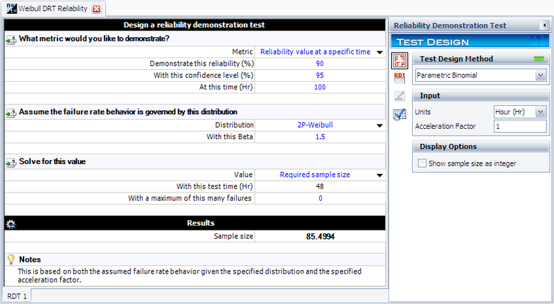
In this example, we will use the parametric binomial method to design a test to demonstrate a reliability of 90% at [math]\displaystyle{ {{t}_{DEMO}}=100\,\! }[/math] hours with a 95% confidence if no failure occur during the test. We will assume a Weibull distribution with a shape parameter [math]\displaystyle{ \beta =1.5\,\! }[/math].

Determining Units for Available Test Time

In the above scenario, we know that we have the testing facilities available for [math]\displaystyle{ t=48\,\! }[/math] hours. We must now determine the number of units to test for this amount of time with no failures in order to have demonstrated our reliability goal. The first step is to determine the Weibull scale parameter, [math]\displaystyle{ \eta \,\! }[/math]. The Weibull reliability equation is:

[math]\displaystyle{ R={{e}^{-{{(t/\eta )}^{\beta }}}}\,\! }[/math]

This can be rewritten as:

[math]\displaystyle{ \eta =\frac{{{t}_{DEMO}}}{{{(-\text{ln}({{R}_{DEMO}}))}^{\tfrac{1}{\beta }}}}\,\! }[/math]

Since we know the values of [math]\displaystyle{ {{t}_{DEMO}}\,\! }[/math], [math]\displaystyle{ {{R}_{DEMO}}\,\! }[/math] and [math]\displaystyle{ \beta \,\! }[/math], we can substitute these in the equation and solve for [math]\displaystyle{ \eta \,\! }[/math]:

[math]\displaystyle{ \eta =\frac{100}{{{(-\text{ln}(0.9))}^{\tfrac{1}{1.5}}}}=448.3\,\! }[/math]

Next, the value of [math]\displaystyle{ {{R}_{TEST}}\,\! }[/math] is calculated by:

[math]\displaystyle{ {{R}_{TEST}}={{e}^{-{{({{t}_{TEST}}/\eta )}^{\beta }}}}={{e}^{-{{(48/448.3)}^{1.5}}}}=0.966=96.6%\,\! }[/math]

The last step is to substitute the appropriate values into the cumulative binomial equation, which for the Weibull distribution appears as:

[math]\displaystyle{ 1-CL=\underset{i=0}{\overset{f}{\mathop \sum }}\,\frac{n!}{i!\cdot (n-i)!}\cdot {{(1-{{e}^{-{{({{t}_{TEST}}/\eta )}^{\beta }}}})}^{i}}\cdot {{({{e}^{-{{({{t}_{TEST}}/\eta )}^{\beta }}}})}^{(n-i)}}\,\! }[/math]

The values of [math]\displaystyle{ CL\,\! }[/math], [math]\displaystyle{ {{t}_{TEST}}\,\! }[/math], [math]\displaystyle{ \beta \,\! }[/math], [math]\displaystyle{ f\,\! }[/math] and [math]\displaystyle{ \eta \,\! }[/math] have already been calculated or specified, so it merely remains to solve the equation for [math]\displaystyle{ n\,\! }[/math]. This value is [math]\displaystyle{ n=85.4994\,\! }[/math], or [math]\displaystyle{ n=86\,\! }[/math] units, since the fractional value must be rounded up to the next integer value. This example solved in Weibull++ is shown next.

Determining Time for Available Units

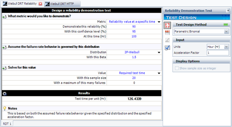
In this case, we will assume that we have 20 units to test, [math]\displaystyle{ n=20\,\! }[/math], and must determine the test time, [math]\displaystyle{ {{t}_{TEST}}\,\! }[/math]. We have already determined the value of the scale parameter, [math]\displaystyle{ \eta \,\! }[/math], in the previous example. Since we know the values of [math]\displaystyle{ n\,\! }[/math], [math]\displaystyle{ CL\,\! }[/math], [math]\displaystyle{ f\,\! }[/math], [math]\displaystyle{ \eta \,\! }[/math] and [math]\displaystyle{ \beta \,\! }[/math], it remains to solve the binomial equation with the Weibull distribution for [math]\displaystyle{ {{t}_{TEST}}\,\! }[/math]. This value is [math]\displaystyle{ {{t}_{TEST}}=126.4339\,\! }[/math] hours. This example solved in Weibull++ is shown next.

Test to Demonstrate MTTF

Designing a test to demonstrate a certain value of the [math]\displaystyle{ MTTF }[/math] is identical to designing a reliability demonstration test, with the exception of how the value of the scale parameter [math]\displaystyle{ \phi \,\! }[/math] is determined. Given the value of the [math]\displaystyle{ MTTF }[/math] and the value of the shape parameter [math]\displaystyle{ \theta \,\! }[/math] , the value of the scale parameter [math]\displaystyle{ \phi \,\! }[/math] can be calculated. With this, the analysis can proceed as with the reliability demonstration methodology.

Example

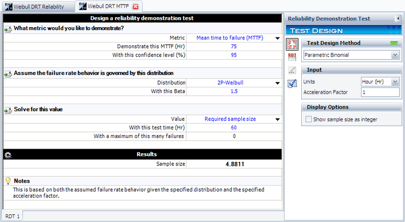
In this example, we will use the parametric binomial method to design a test that will demonstrate [math]\displaystyle{ MTTF=75\,\! }[/math] hours with a 95% confidence if no failure occur during the test [math]\displaystyle{ f=0\,\! }[/math]. We will assume a Weibull distribution with a shape parameter [math]\displaystyle{ \beta =1.5\,\! }[/math]. We want to determine the number of units to test for [math]\displaystyle{ {{t}_{TEST}}=60\,\! }[/math] hours to demonstrate this goal.

The first step in this case involves determining the value of the scale parameter [math]\displaystyle{ \eta \,\! }[/math] from the [math]\displaystyle{ MTTF\,\! }[/math] equation. The equation for the [math]\displaystyle{ MTTF\,\! }[/math] for the Weibull distribution is:

[math]\displaystyle{ MTTF=\eta \cdot \Gamma (1+\frac{1}{\beta })\,\! }[/math]

where [math]\displaystyle{ \Gamma (x)\,\! }[/math] is the gamma function of [math]\displaystyle{ x\,\! }[/math]. This can be rearranged in terms of [math]\displaystyle{ \eta\,\! }[/math]:

[math]\displaystyle{ \eta =\frac{MTTF}{\Gamma (1+\tfrac{1}{\beta })}\,\! }[/math]

Since [math]\displaystyle{ MTTF\,\! }[/math] and [math]\displaystyle{ \beta \,\! }[/math] have been specified, it is a relatively simple matter to calculate [math]\displaystyle{ \eta =83.1\,\! }[/math]. From this point on, the procedure is the same as the reliability demonstration example. Next, the value of [math]\displaystyle{ {{R}_{TEST}}\,\! }[/math] is calculated as:

[math]\displaystyle{ {{R}_{TEST}}={{e}^{-{{({{t}_{TEST}}/\eta )}^{\beta }}}}={{e}^{-{{(60/83.1)}^{1.5}}}}=0.541=54.1%\,\! }[/math]

The last step is to substitute the appropriate values into the cumulative binomial equation. The values of [math]\displaystyle{ CL\,\! }[/math], [math]\displaystyle{ {{t}_{TEST}}\,\! }[/math], [math]\displaystyle{ \beta \,\! }[/math], [math]\displaystyle{ f\,\! }[/math] and [math]\displaystyle{ \eta \,\! }[/math] have already been calculated or specified, so it merely remains to solve the binomial equation for [math]\displaystyle{ n\,\! }[/math]. The value is calculated as [math]\displaystyle{ n=4.8811,\,\! }[/math] or [math]\displaystyle{ n=5\,\! }[/math] units, since the fractional value must be rounded up to the next integer value. This example solved in Weibull++ is shown next.

The procedure for determining the required test time proceeds in the same manner, determining [math]\displaystyle{ \eta \,\! }[/math] from the [math]\displaystyle{ MTTF\,\! }[/math] equation, and following the previously described methodology to determine [math]\displaystyle{ {{t}_{TEST}}\,\! }[/math] from the binomial equation with Weibull distribution.

Non-Parametric Binomial

The binomial equation can also be used for non-parametric demonstration test design. There is no time value associated with this methodology, so one must assume that the value of [math]\displaystyle{ {{R}_{TEST}}\,\! }[/math] is associated with the amount of time for which the units were tested.

In other words, in cases where the available test time is equal to the demonstration time, the following non-parametric binomial equation is widely used in practice:

[math]\displaystyle{ \begin{align} 1-CL=\sum_{i=0}^{f}\binom{n}{i}(1-{{R}_{TEST}})^{i}{{R}_{TEST}}^{n-i} \end{align} }[/math]

where [math]\displaystyle{ CL\,\! }[/math] is the confidence level, [math]\displaystyle{ f\,\! }[/math] is the number of failures, [math]\displaystyle{ n\,\! }[/math] is the sample size and [math]\displaystyle{ {{R}_{TEST}}\,\! }[/math] is the demonstrated reliability. Given any three of them, the remaining one can be solved for.

Non-parametric demonstration test design is also often used for one shot devices where the reliability is not related to time. In this case, [math]\displaystyle{ {{R}_{TEST}}\,\! }[/math] can be simply written as [math]\displaystyle{ {R}\,\! }[/math].

Example

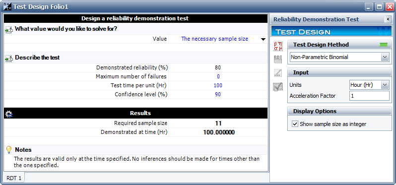
A reliability engineer wants to design a zero-failure demonstration test in order to demonstrate a reliability of 80% at a 90% confidence level. Use the non-parametric binomial method to determine the required sample size.

Solution

By substituting [math]\displaystyle{ f=0\,\! }[/math] (since it a zero-failure test) the non-parametric binomial equation becomes:

[math]\displaystyle{ \begin{align} 1-CL=R^{n} \end{align}\,\! }[/math]

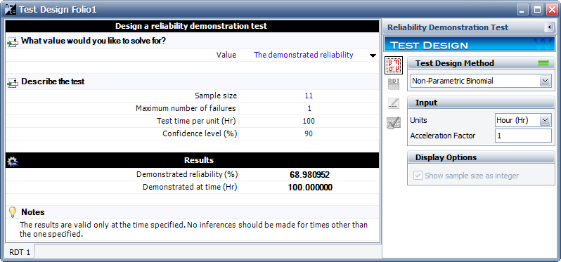
So now the required sample size can be easily solved for any required reliability and confidence level. The result of this test design was obtained using Weibull++ and is:

The result shows that 11 samples are needed. Note that the time value shown in the above figure is chance indicative and not part of the test design (the "Test time per unit" that was input will be the same as the "Demonstrated at time" value for the results). If those 11 samples are run for the required demonstration time and no failures are observed, then a reliability of 80% with a 90% confidence level has been demonstrated. If the reliability of the system is less than or equal to 80%, the chance of passing this test is 1-CL = 0.1, which is the Type II error. Therefore, the non-parametric binomial equation determines the sample size by controlling for the Type II error.

If 11 samples are used and one failure is observed by the end of the test, then the demonstrated reliability will be less than required. The demonstrated reliability is 68.98% as shown below.

Constant Failure Rate/Chi-Squared

Another method for designing tests for products that have an assumed constant failure rate, or exponential life distribution, draws on the chi-squared distribution. These represent the true exponential distribution confidence bounds referred to in The Exponential Distribution. This method only returns the necessary accumulated test time for a demonstrated reliability or [math]\displaystyle{ MTTF\,\! }[/math] , not a specific time/test unit combination that is obtained using the cumulative binomial method described above. The accumulated test time is equal to the total amount of time experienced by all of the units on test. Assuming that the units undergo the same amount of test time, this works out to be:

[math]\displaystyle{ {{T}_{a}}=n\cdot {{t}_{TEST}} }[/math]

where [math]\displaystyle{ n\,\! }[/math] is the number of units on test and [math]\displaystyle{ {{t}_{TEST}}\,\! }[/math] is the test time. The chi-squared equation for test time is:

[math]\displaystyle{ {{T}_{a}}=\frac{MTTF\cdot \chi _{1-CL;2f+2}^{2}}{2} }[/math]

where:

• [math]\displaystyle{ \chi _{1-CL;2f+2}^{2}\,\! }[/math] = the chi-squared distribution
• [math]\displaystyle{ {{T}_{a}}\,\! }[/math] = the necessary accumulated test time
• [math]\displaystyle{ CL\,\! }[/math] = the confidence level
• [math]\displaystyle{ f\,\! }[/math] = the number of failures

Since this methodology only applies to the exponential distribution, the exponential reliability equation can be rewritten as:

[math]\displaystyle{ MTTF=\frac{t}{-ln(R)} }[/math]

and substituted into the chi-squared equation for developing a test that demonstrates reliability at a given time, rather than [math]\displaystyle{ MTTF\,\! }[/math] :

[math]\displaystyle{ {{T}_{a}}=\frac{\tfrac{{{t}_{DEMO}}}{-ln(R)}\cdot \chi _{1-CL;2f+2}^{2}}{2} }[/math]

Example

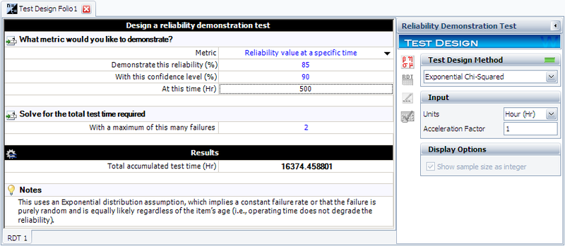
In this example, we will use the exponential chi-squared method to design a test that will demonstrate a reliability of 85% at [math]\displaystyle{ {{t}_{DEMO}}=500\,\! }[/math] hours with a 90% confidence (or [math]\displaystyle{ CL=0.9\,\! }[/math]) if no more than 2 failures occur during the test ([math]\displaystyle{ f=2\,\! }[/math]). The chi-squared value can be determined from tables or the Quick Statistical Reference (QSR) tool in Weibull++. In this example, the value is calculated as:

[math]\displaystyle{ \chi _{1-CL;2r+2}^{2}=\chi _{0.1;6}^{2}=10.6446\,\! }[/math]

Substituting this into the chi-squared equation, we obtain:

[math]\displaystyle{ {{T}_{a}}=\frac{\tfrac{500}{-ln(0.85)}\cdot 10.6446}{2}=16,374\text{ hours}\,\! }[/math]

This means that 16,374 hours of total test time needs to be accumulated with no more than two failures in order to demonstrate the specified reliability.

This example solved in Weibull++ is shown next.

Given the test time, one can now solve for the number of units using the chi-squared equation. Similarly, if the number of units is given, one can determine the test time from the chi-squared equation for exponential test design.

Bayesian Non-Parametric Test Design

The regular non-parametric analyses performed based on either the binomial or the chi-squared equation were performed with only the direct system test data. However, if prior information regarding system performance is available, it can be incorporated into a Bayesian non-parametric analysis. This subsection will demonstrate how to incorporate prior information about system reliability and also how to incorporate prior information from subsystem tests into system test design.

If we assume the system reliability follows a beta distribution, the values of system reliability, R, confidence level, CL, number of units tested, n, and number of failures, r, are related by the following equation:

[math]\displaystyle{ 1-CL=\text{Beta}\left(R,\alpha,\beta\right)=\text{Beta}\left(R,n-r+\alpha_{0},r+\beta_{0}\right) }[/math]

where [math]\displaystyle{ Beta\,\! }[/math] is the incomplete beta function. If [math]\displaystyle{ {{\alpha}_{0}} \gt 0\,\! }[/math] and [math]\displaystyle{ {{\beta}_{0}} \gt 0\,\! }[/math] are known, then any quantity of interest can be calculated using the remaining three. The next two examples demonstrate how to calculate [math]\displaystyle{ {{\alpha}_{0}} \gt 0\,\! }[/math] and [math]\displaystyle{ {{\beta}_{0}} \gt 0\,\! }[/math] depending on the type of prior information available.

Use Prior Expert Opinion on System Reliability

Prior information on system reliability can be exploited to determine [math]\displaystyle{ \alpha_{0}\,\! }[/math] and [math]\displaystyle{ \beta_{0}\,\! }[/math]. To do so, first approximate the expected value and variance of prior system reliability [math]\displaystyle{ R_{0}\,\! }[/math]. This requires knowledge of the lowest possible reliability, the most likely possible reliability and the highest possible reliability of the system. These quantities will be referred to as a, b and c, respectively. The expected value of the prior system reliability is approximately given as:

[math]\displaystyle{ E\left(R_{0}\right)=\frac{a+4b+c}{6} }[/math]

and the variance is approximately given by:

[math]\displaystyle{ Var({{R}_{0}})={{\left( \frac{c-a}{6} \right)}^{2}} }[/math]

These approximate values of the expected value and variance of the prior system reliability can then be used to estimate the values of [math]\displaystyle{ \alpha_{0}\,\! }[/math] and [math]\displaystyle{ \beta_{0}\,\! }[/math], assuming that the prior reliability is a beta-distributed random variable. The values of [math]\displaystyle{ \alpha_{0}\,\! }[/math] and [math]\displaystyle{ \beta_{0}\,\! }[/math] are calculated as:

[math]\displaystyle{ \alpha_{0}=E\left(R_{0}\right)\left[\frac{E\left(R_{0}\right)-E^{2}\left(R_{0}\right)}{Var\left(R_{0}\right)}-1\right] }[/math] [math]\displaystyle{ \beta_{0}=\left(1-E\left(R_{0}\right)\right)\left[\frac{E\left(R_{0}\right)-E^{2}\left(R_{0}\right)}{Var\left(R_{0}\right)}-1\right] }[/math]

With [math]\displaystyle{ \alpha_{0}\,\! }[/math] and [math]\displaystyle{ \beta_{0}\,\! }[/math] known, the above beta distribution equation can now be used to calculate a quantity of interest.

Example

You can use the non-parametric Bayesian method to design a test using prior knowledge about a system's reliability. For example, suppose you wanted to know the reliability of a system and you had the following prior knowledge of the system:

• Lowest possible reliability: a = 0.8

• Most likely reliability: b = 0.85

• Highest possible reliability: c = 0.97

This information can be used to approximate the expected value and the variance of the prior system reliability.

[math]\displaystyle{ E\left(R_{0}\right)=\frac{a+4b+c}{6}=0.861667 \,\! }[/math]

[math]\displaystyle{ Var({{R}_{0}})={{\left( \frac{c-a}{6} \right)}^{2}}=0.000803 \,\! }[/math]

These approximations of the expected value and variance of the prior system reliability can then be used to estimate [math]\displaystyle{ \alpha_{0}\,\! }[/math] and [math]\displaystyle{ \beta_{0}\,\! }[/math] used in the beta distribution for the system reliability, as given next:

[math]\displaystyle{ \alpha\,\!_{0}=E\left(R_{0}\right)\left[\frac{E\left(R_{0}\right)-E^{2}\left(R_{0}\right)}{Var\left(R_{0}\right)}-1\right]=127.0794\,\! }[/math]

[math]\displaystyle{ \beta\,\!_{0}=\left(1-E\left(R_{0}\right)\right)\left[\frac{E\left(R_{0}\right)-E^{2}\left(R_{0}\right)}{Var\left(R_{0}\right)}-1\right]=20.40153\,\! }[/math]

With [math]\displaystyle{ \alpha_{0}\,\! }[/math] and [math]\displaystyle{ \beta_{0}\,\! }[/math] known, any single value of the four quantities system reliability R, confidence level CL, number of units n, or number of failures r can be calculated from the other three using the beta distribution function:

[math]\displaystyle{ 1-CL=\text{Beta}\left(R,\alpha,\beta\right)=\text{Beta}\left(R,n-r+\alpha_{0},r+\beta_{0}\right)\,\! }[/math]

Solve for System Reliability R

Given CL = 0.9, n = 20, and r = 1, using the above prior information to solve R.

First, we get the number of successes: s = n – r = 19. Then the parameters in the posterior beta distribution for R are calculated as:

[math]\displaystyle{ \alpha\,\!=\alpha\,\!_{0}+s=146.0794\,\! }[/math]

[math]\displaystyle{ \beta\,\!=\beta\,\!_{0}+r=21.40153\,\! }[/math]

Finally, from this posterior distribution, the system reliability R at a confidence level of CL=0.9 is solved as:

[math]\displaystyle{ R=\text{BetaINV}\left(1-CL,\alpha\,\!,\beta\,\!\right)=0.838374 \,\! }[/math]

Solve for Confidence Level CL

Given R = 0.85, n = 20, and r = 1, using the above prior information on system reliability to solve for CL.

First, we get the number of successes: s = n – r = 19. Then the parameters in the posterior beta distribution for R are calculated as:

[math]\displaystyle{ \alpha\,\!=\alpha\,\!_{0}+s=146.07943\,\! }[/math]

[math]\displaystyle{ \beta\,\!=\beta\,\!_{0}+r=21.40153\,\! }[/math]

Finally, from this posterior distribution, the corresponding confidence level for reliability R=0.85 is:

[math]\displaystyle{ CL=\text{Beta}\left(R,\alpha,\beta\right)=0.81011 \,\! }[/math]

Solve for Sample Size n

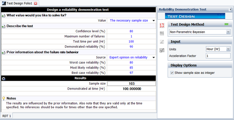
Given R = 0.9, CL = 0.8, and r = 1, using the above prior information on system reliability to solve the required sample size in the demonstration test.

Again, the above beta distribution equation for the system reliability can be utilized. The figure below shows the result from Weibull++. The results show that the required sample size is 103. Weibull++ always displays the sample size as an integer.

Use Prior Information from Subsystem Tests

Prior information from subsystem tests can also be used to determine values of alpha and beta. Information from subsystem tests can be used to calculate the expected value and variance of the reliability of individual components, which can then be used to calculate the expected value and variance of the reliability of the entire system. [math]\displaystyle{ \alpha_{0}\,\! }[/math] and [math]\displaystyle{ \beta_{0}\,\! }[/math] are then calculated as before:

[math]\displaystyle{ \alpha_{0}=E\left(R_{0}\right)\left[\frac{E\left(R_{0}\right)-E^{2}\left(R_{0}\right)}{Var\left(R_{0}\right)}-1\right] }[/math]

[math]\displaystyle{ \beta_{0}=\left(1-E\left(R_{0}\right)\right)\left[\frac{E\left(R_{0}\right)-E^{2}\left(R_{0}\right)}{Var\left(R_{0}\right)}-1\right] }[/math]

For each subsystem i, from the beta distribution, we can calculate the expected value and the variance of the subsystem’s reliability [math]\displaystyle{ R_{i}\,\! }[/math] as [38]:

[math]\displaystyle{ E\left(R_{i}\right)=\frac{s_{i}}{n_{i}+1} }[/math]

[math]\displaystyle{ Var\left(R_{i}\right)=\frac{s_{i}\left(n_{i}+1-s_{i}\right)}{\left(n_{i}+1\right)^{2}\left(n_{i}+2\right)} }[/math]

Assuming that all the subsystems are in a series reliability-wise configuration, the expected value and variance of the system’s reliability [math]\displaystyle{ R\,\! }[/math] can then be calculated as [38]:

[math]\displaystyle{ E\left(R_{0}\right)=(i=1)^{k} E\left(R_{i}\right)=E\left(R_{1}\right)\times E\left(R_{2}\right)\ldots E\left(R_{k}\right) }[/math]

[math]\displaystyle{ Var\left(R_{0}\right)=\prod_{i=1}^{k}\left[E^{2}\left(R_{i}\right)+Var\left(R_{i}\right)\right]-\prod_{i=1}^{k}\left[E^{2}\left(R_{i}\right)\right] }[/math]

With the above prior information on the expected value and variance of the system reliability, all the calculations can now be calculated as before.

Example

You can use the non-parametric Bayesian method to design a test for a system using information from tests on its subsystems. For example, suppose a system of interest is composed of three subsystems A, B and C -- with prior information from tests of these subsystems given in the table below.

Subsystem	Number of Units (n)	Number of Failures (r)
A	20	0
B	30	1
C	100	4

This data can be used to calculate the expected value and variance of the reliability for each subsystem.

[math]\displaystyle{ E\left(R_{i}\right)=\frac{n_{i}-r_{i}}{n_{i}+1} \,\! }[/math]

[math]\displaystyle{ Var\left(R_{i}\right)=\frac{\left(n_{i}-r_{i}\right)\left(r_{i}+1\right)}{\left(n_{i}+1\right)^{2}\left(n_{i}+2\right)} \,\! }[/math]

The results of these calculations are given in the table below.

Subsystem	Mean of Reliability	Variance of Reliability
A	0.952380952	0.002061
B	0.935483871	0.001886
C	0.95049505	0.000461

These values can then be used to find the prior system reliability and its variance:

[math]\displaystyle{ E\left(R_{0}\right)=0.846831227\,\! }[/math]

[math]\displaystyle{ \text{Var}\left(R_{0}\right)=0.003546663\,\! }[/math]

From the above two values, the parameters of the prior distribution of the system reliability can be calculated by:

[math]\displaystyle{ \alpha_{0}=E\left(R_{0}\right)\left[\frac{E\left(R_{0}\right)-E^{2}\left(R_{0}\right)}{\text{Var}\left(R_{0}\right)}-1\right]=30.12337003\,\! }[/math]

[math]\displaystyle{ \beta_{0}=\left(1-E \left(R_{0}\right)\right)\left[\frac{E\left(R_{0}\right)-E^{2}\left(R_{0}\right)}{Var \left(R_{0}\right)}-1\right]=5.448499634\,\! }[/math]

With this prior distribution, we now can design a system reliability demonstration test by calculating system reliability R, confidence level CL, number of units n or number of failures r, as needed.

Solve for Sample Size n

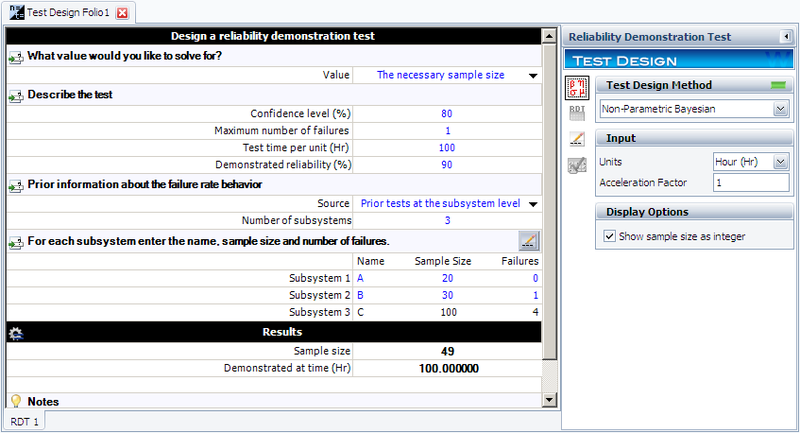
Given the above subsystem test information, in order to demonstrate the system reliability of 0.9 at a confidence level of 0.8, how many samples are needed in the test? Assume the allowed number of failures is 1.

Using Weibull++, the results are given in the figure below. The result shows that at least 49 test units are needed.

Expected Failure Times Plots

Test duration is one of the key factors that should be considered in designing a test. If the expected test duration can be estimated prior to the test, test resources can be better allocated. In this section, we will explain how to estimate the expected test time based on test sample size and the assumed underlying failure distribution.

The binomial equation used in non-parametric demonstration test design is the base for predicting expected failure times. The equation is:

[math]\displaystyle{ 1-CL=\underset{i=0}{\overset{r}{\mathop \sum }}\,\frac{n!}{i!\cdot (n-i)!}\cdot {{(1-{{R}_{TEST}})}^{i}}\cdot R_{TEST}^{(n-i)} }[/math]

where:

• [math]\displaystyle{ CL\,\! }[/math] = the required confidence level
• [math]\displaystyle{ r\,\! }[/math] = the number of failures
• [math]\displaystyle{ n\,\! }[/math] = the total number of units on test
• [math]\displaystyle{ {{R}_{TEST}}\,\! }[/math] = the reliability on test

If CL, r and n are given, the R value can be solved from the above equation. When CL=0.5, the solved R (or Q, the probability of failure whose value is 1-R) is the so called median rank for the corresponding failure. (For more information on median ranks, please see Parameter Estimation).

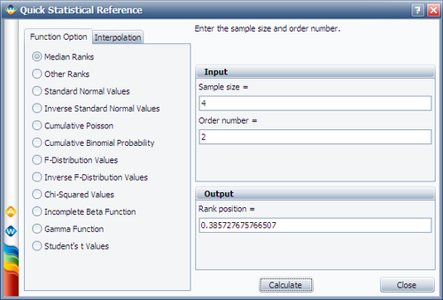
For example, given n = 4, r = 2 and CL = 0.5, the calculated Q is 0.385728. This means, at the time when the second failure occurs, the estimated system probability of failure is 0.385728. The median rank can be calculated in Weibull++ using the Quick Statistical Reference, as shown below:

Similarly, if we set r = 3 for the above example, we can get the probability of failure at the time when the third failure occurs. Using the estimated median rank for each failure and the assumed underlying failure distribution, we can calculate the expected time for each failure. Assume the failure distribution is Weibull, then we know:

[math]\displaystyle{ Q=1-{{e}^-{{{\left( \frac{t}{\eta } \right)}^{\beta }}}} }[/math]

where:

• [math]\displaystyle{ \beta \,\! }[/math] is the shape parameter
• [math]\displaystyle{ \eta\,\! }[/math] is the scale parameter

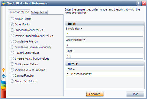
Using the above equation, for a given Q, we can get the corresponding time t. The above calculation gives the median of each failure time for CL = 0.5. If we set CL at different values, the confidence bounds of each failure time can be obtained. For the above example, if we set CL=0.9, from the calculated Q we can get the upper bound of the time for each failure. The calculated Q is given in the next figure:

If we set CL=0.1, from the calculated Q we can get the lower bound of the time for each failure. The calculated Q is given in the figure below:

Example

In this example you will use the Expected Failure Times plot to estimate the duration of a planned reliability test. 4 units were allocated for the test, and the test engineers want to know how long the test will last if all the units are tested to failure. Based on previous experiments, they assume the underlying failure distribution is a Weibull distribution with [math]\displaystyle{ \beta = 2\,\! }[/math] and [math]\displaystyle{ \eta = 500\,\! }[/math].

Solution

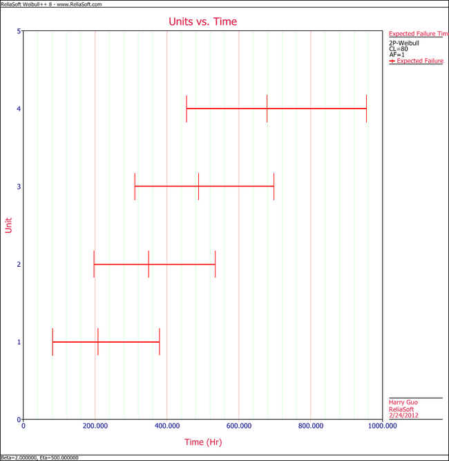
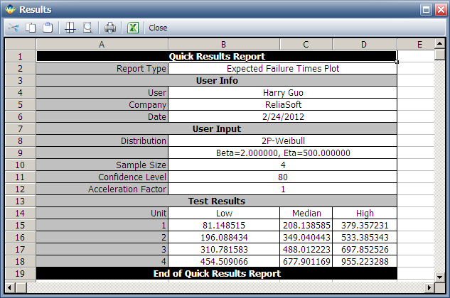
Using Weibull++'s Expected Failure Times plot, the expected failure times with 80% 2-sided confidence bounds are given below.

From the above results, we can see the upper bound of the last failure is about 955 hours. Therefore, the test probably will last for around 955 hours.

As we know, with 4 samples, the median rank for the second failure is 0.385728. Using this value and the assumed Weibull distribution, the median value of the failure time of the second failure is calculated as:

[math]\displaystyle{ \begin{align} & Q=1-{{e}^-{{{\left( \frac{t}{\eta } \right)}^{\beta }}}}\Rightarrow \\ & \ln (1-Q)={{\left( \frac{t}{\eta } \right)}^{\beta }} \\ & \Rightarrow t=\text{349.04}\\ \end{align}\,\! }[/math]

Its bounds and other failure times can be calculated in a similar way.

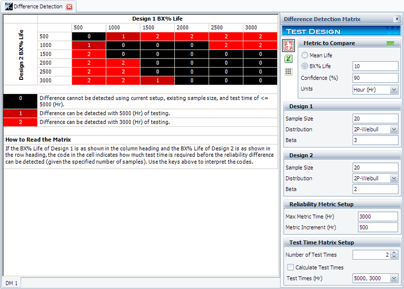
Life Difference Detection Matrix

Engineers often need to design tests for detecting life differences between two or more product designs. The questions are how many samples and how long should the test be conducted in order to detect a certain amount of difference. There are no simple answers. Usually, advanced design of experiments (DOE) techniques should be utilized. For a simple case, such as comparing two designs, the Difference Detection Matrix in Weibull++ can be used. The Dfference Detection Matrix graphically indicates the amount of test time required to detect a statistical difference in the lives of two populations.

As discussed in the test design using Expected Failure Times plot, if the sample size is known, the expected failure time of each test unit can be obtained based on the assumed failure distribution. Now let's go one step further. With these failure times, we can then estimate the failure distribution and calculate any reliability metrics. This process is similar to the simulation used in SimuMatic where random failure times are generated from simulation and then used to estimate the failure distribution. This approach is also used by the Difference Detection Matrix.

Assume we want to compare the B10 lives (or mean lives) of two designs. The test is time-terminated and the termination time is set to T. Using the method given in Expected Failure Times Plots, we can generate the failure times. For any failure time greater than T, it is a suspension and the suspension time is T. For each design, its B10 life and confidence bounds can be estimated from the generated failure/suspension times. If the two estimated confidence intervals overlap with each other, it means the difference of the two B10 lives cannot be detected from this test. We have to either increase the sample size or the test duration.

Example

In this example, you will use the Difference Detection Matrix to choose the suitable sample size and duration for a reliability test. Assume that there are two design options for a new product. The engineers need to design a test that compares the reliability performance of these two options. The reliability for both designs is assumed to follow a Weibull distribution. For Design 1, its shape parameter [math]\displaystyle{ \beta = 3\,\! }[/math]; for Design 2, its [math]\displaystyle{ \beta= 2\,\! }[/math]. Their B10 lives may range from 500 to 3,000 hours.

Solution

For the initial setup, set the sample size for each design to 20, and use two test durations of 3,000 and 5,000 hours. The following picture shows the complete control panel setup and the results of the analysis.

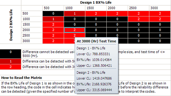
The columns in the matrix show the range of the assumed B10 life for design 1, while the rows show the range for design 2. A value of 0 means the difference cannot be detected through the test, 1 means the difference can be detected if the test duration is 5,000 hours, and 2 means the difference can be detected if the test duration is 3,000 hours. For example, the number is 2 for cell (1000, 2000). This means that if the B10 life for Design 1 is 1,000 hours and the B10 life for Design 2 is 2,000 hours, the difference can be detected if the test duration is at least 5,000 hours.

Click inside the cell to show the estimated confidence intervals, as shown next. By testing 20 samples each for 3,000 hours, the difference of their B10 lives probably can be detected. This is because, at a confidence level of 90%, the estimated confidence intervals on the B10 life do not overlap.

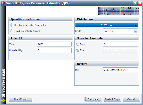
We will use Design 1 to illustrate how the interval is calculated. For cell (1000, 2000), Design 1's B10 life is 1,000 and the assumed [math]\displaystyle{ \beta\,\! }[/math] is 3. We can calculate the [math]\displaystyle{ \eta\,\! }[/math] for the Weibull distribution using the Quick Parameter Estimator tool, as shown next.

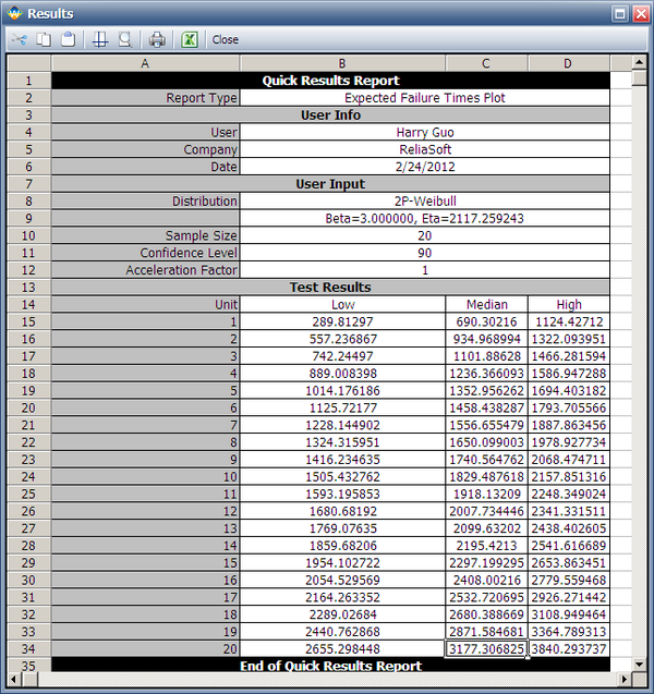
The estimated [math]\displaystyle{ \eta\,\! }[/math] is 2117.2592 hours. We can then use these distribution parameters and the sample size of 20 to get the expected failure times by using Weibull's Expected Failure Times Plot. The following report shows the result from that utility.

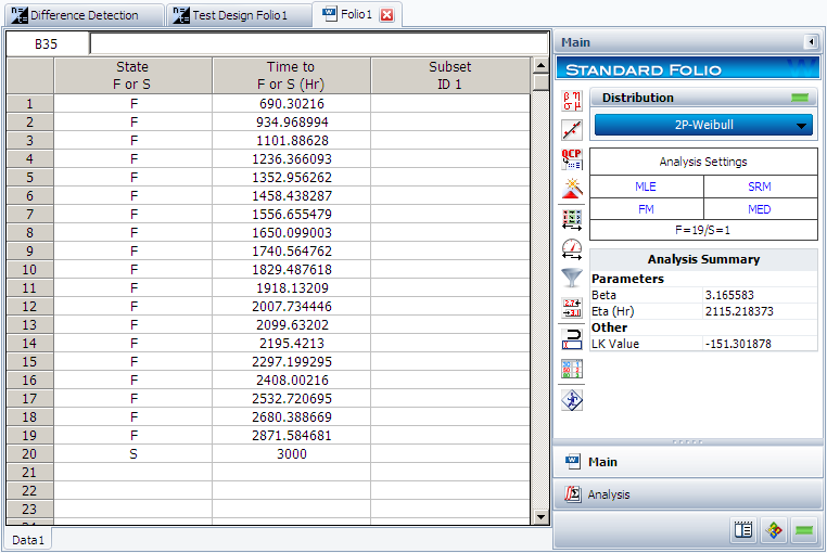
The median failure times are used to estimate the failure distribution. Note that since the test duration is set to 3,000 hours, any failures that occur after 3,000 are treated as suspensions. In this case, the last failure is a suspension with a suspension time of 3,000 hours. We can enter the median failure times data set into a standard Weibull++ folio as given in the next figure.

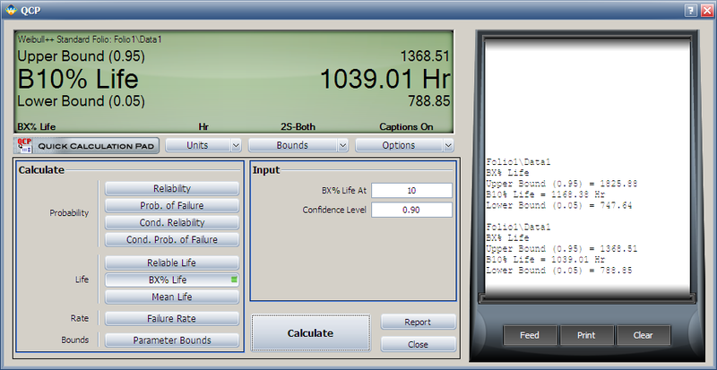
After analyzing the data set with the MLE and FM analysis options, we can now calculate the B10 life and its interval in the QCP, as shown next.

From this result, we can see that the estimated B10 life and its confidence intervals are the same as the results displayed in the Difference Detection Matrix.

The above procedure can be repeated to get the results for the other cells and for Design 2. Therefore, by adjusting the sample size and test duration, a suitable test time can be identified for detecting a certain amount of difference between two designs/populations.

Simulation

Monte Carlo simulation provides another useful tool for test design. The SimuMatic utility in Weibull++ can be used for this purpose. SimuMatic is simulating the outcome from a particular test design that is intended to demonstrate a target reliability. You can specify various factors of the design, such as the test duration (for a time-terminated test), number of failures (for a failure-terminated test) and sample size. By running the simulations you can assess whether the planned test design can achieve the reliability target. Depending on the results, you can modify the design by adjusting these factors and repeating the simulation process—in effect, simulating a modified test design—until you arrive at a modified design that is capable of demonstrating the target reliability within the available time and sample size constraints.

Of course, all the design factors mentioned in SimuMatic also can be calculated using analytical methods as discussed in previous sections. However, all of the analytical methods need assumptions. When sample size is small or test duration is short, these assumptions may not be accurate enough. The simulation method usually does not require any assumptions. For example, the confidence bounds of reliability from SimuMatic are purely based on simulation results. In analytical methods, both Fisher bounds and likelihood ratio bounds need to use assumptions. Another advantage of using the simulation method is that it is straightforward and results can be visually displayed in SimuMatic.

For details, see the Weibull++ SimuMatic chapter.