Failure Discounting

During a reliability growth test, once a failure has been analyzed and corrective actions for that specific failure mode have been implemented, the probability of its recurrence is diminished [4]. Then for the success/failure data that follow, the value of the failure for which corrective actions have already been implemented should be subtracted from the total number of failures. But certain questions arise, such as, To what extent should the failure value be diminished or discounted? and How should the failure value be defined? One answer would be to use engineering judgment, (e.g., a panel of specialists would agree that the probability of failure has been reduced by 50% or 90% and therefore that failure should be given a value of 0.5 or 0.9). The obvious disadvantage of this approach is its arbitrariness and the difficulty of reaching an agreement. Therefore, a statistical basis is selected, one that is repeatable and less arbitrary. Failure discounting is applied when using the Lloyd-Lipow, Logistic and the Standard and Modified Gompertz models.

The value of the failure, [math]\displaystyle{ f\,\! }[/math] , is chosen to be the upper confidence limit on the probability of failure based on the number of successful tests following implementation of the corrective action. The failure value is given by the following equation:

[math]\displaystyle{ f=1-{{(1-CL)}^{\tfrac{1}{{{S}_{n}}}}} }[/math]

where:

[math]\displaystyle{ \begin{align} & CL= & \text{the confidence level}\text{.} \\ & {{S}_{n}}= & \text{the number of successful tests after the first success } \\ & & \text{following the corrective action}\text{.} \end{align} }[/math]

For example, after one successful test following a corrective action, [math]\displaystyle{ {{S}_{n}}=1\,\! }[/math] , the failure is given a value of 0.9 based on a 90% confidence level. After two successful tests, [math]\displaystyle{ {{S}_{n}}=2\,\! }[/math] , the failure is given a value of 0.684, and so on. The procedure for applying this method is illustrated in the next example.

Example

Use failure discounting to answer the questions below. Assume that during the 22 launches given in the first table below, the first failure was caused by Mode 1, the second and fourth failures were caused by Mode 2, the third and fifth failures were caused by Mode 3, the sixth failure was caused by Mode 4 and the seventh failure was caused by Mode 5.

1) Find the Standard Gompertz reliability growth curve using the results of the first 15 launches.

2) Find the predicted reliability after launch 22.

3) Calculate the reliability after launch 22 based on the full data set from the second table and compare with the estimate obtained for question 2.

Launch sequence with failure modes and failure values
Launch Number	Result/Mode	Failure 1	Failure 2	Failure 3	Failure 4	Failure 5	Failure 6	Failure 7	Sum of Failures
1	F1	1.000							1.000
2	F2	1.000	1.000						2.000
3	F3	0.900	1.000	1.000					2.900
4	S	0.684	0.900	1.000					2.584
5	F2	0.536	1.000	0.900	1.000				3.436
6	F3	0.438	1.000	1.000	1.000	1.000			4.438
7	S	0.369	0.900	1.000	0.900	1.000			4.169
8	S	0.319	0.684	0.900	0.684	0.900			3.486
9	S	0.280	0.536	0.684	0.536	0.684			2.720
10	S	0.250	0.438	0.536	0.438	0.536			2.197
11	S	0.226	0.369	0.438	0.369	0.438			1.839
12	S	0.206	0.319	0.369	0.319	0.369			1.581
13	S	0.189	0.280	0.319	0.280	0.319			1.387
14	S	0.175	0.250	0.280	0.250	0.280			1.235
15	S	0.162	0.226	0.250	0.226	0.250			1.114
16	S	0.152	0.206	0.226	0.206	0.226			1.014
17	F4	0.142	0.189	0.206	0.189	0.206	1.000		1.931
18	S	0.134	0.175	0.189	0.175	0.189	1.000		1.861
19	F5	0.127	0.162	0.175	0.162	0.175	0.900	1.000	2.701
20	S	0.120	0.152	0.162	0.152	0.162	0.684	1.000	2.432
21	S	0.114	0.142	0.152	0.142	0.152	0.536	0.900	2.138
22	S	0.109	0.134	0.142	0.134	0.142	0.438	0.684	1.783

Comparison of the predicted reliability with the actual data
Launch Number	Calculated Reliability (%)	ln(R)	Gompertz Reliability (%)
1	0.000
2	0.000
3	3.333	1.204
4	35.406	3.567	16.426
5	31.283	3.443	26.691
6	26.039	3.260	37.858
7	40.442	3.670	48.691
8	56.422	4.033	58.363
9	69.783	4.245	66.496
		[math]\displaystyle{ {{S}_{1}} }[/math] = 22.218
10	78.029	4.357	73.044
11	83.281	4.422	78.155
12	86.824	4.464	82.055
13	89.331	4.492	84.983
14	91.175	4.513	87.155
15	92.573	4.528	88.754
		[math]\displaystyle{ {{S}_{2}} }[/math] = 26.776
16	93.660	4.540	89.923
17	88.639	4.484	90.774
18	89.661	4.496	91.392
19	85.787	4.452	91.839
20	87.841	4.476	92.163
21	89.820	4.498	92.396
		[math]\displaystyle{ {{S}_{3}} }[/math] = 26.946
22	91.896 4.521 92.565

Solution

1) The first table above is organized as follows:

• Each failure is represented by a single column and named Failure 1, Failure 2 etc. The failure mode for each failure is shown in the Result/Mode column where is also indicated in the launch is a success.
• The values of failure are calculated from the equation above and are based on [math]\displaystyle{ CL=0.90 }[/math] .
• These values are summed and the reliability is calculated from:

[math]\displaystyle{ R=\left[ 1-\left( \frac{\mathop{}_{i=1}^{N}{{f}_{i}}}{n} \right) \right]\cdot 100\text{ }% }[/math]

where [math]\displaystyle{ N }[/math] is the number of failures and [math]\displaystyle{ n }[/math] is the number of events, tests, runs or launches.

• Failure 1 is Mode 1; it occurs at launch 1 and it does not recur throughout the process.

So at launch 3, [math]\displaystyle{ {{S}_{n}}=1 }[/math] , and so on.

• Failure 2 is Mode 2; it occurs at launch 2 and it recurs at launch 5. Therefore, [math]\displaystyle{ {{S}_{n}}=1 }[/math] at launch 4 and at launch 7, and so on.
• Failure 3 is Mode 3; it occurs at launch 3 and it recurs at launch 6. Therefore, [math]\displaystyle{ {{S}_{n}}=1 }[/math] at launch 5 and at launch 8, and so on.
• Failure 6 is Mode 4; it occurs at launch 17 and it does not recur throughout the process. So at launch 19, [math]\displaystyle{ {{S}_{n}}=1 }[/math] , and so on.
• Failure 7 is Mode 5; it occurs at launch 19 and it does not recur throughout the process. So at launch 21, [math]\displaystyle{ {{S}_{n}}=1 }[/math] , and so on.

For launch 3 and failure 1, [math]\displaystyle{ {{S}_{n}}=1 }[/math].

[math]\displaystyle{ {{f}_{1/3}}=1-{{(1-0.90)}^{1/1}}=0.900 }[/math]

For launch 4 and failure 1, [math]\displaystyle{ {{S}_{n}}=2 }[/math].

[math]\displaystyle{ {{f}_{1/4}}=1-{{(1-0.90)}^{1/2}}=0.684 }[/math]

And so on.

Calculate the initial values of the Gompertz parameters using the second table above. Based on the equations from the Gompertz Models chapter, the initial values are:

<INSERT EQUATION>

Now, since the initial values have been determined, the Gauss-Newton method can be used. Substituting [math]\displaystyle{ {{Y}_{i}}={{R}_{i}}, }[/math] [math]\displaystyle{ g_{1}^{(0)}=89.31, }[/math] [math]\displaystyle{ g_{2}^{(0)}=0.127, }[/math] [math]\displaystyle{ g_{3}^{(0)}=0.578 }[/math] . The iterations are continued to solve for the parameters. Using the RGA software, the estimators of the parameters for the given example are:

[math]\displaystyle{ \begin{align} & \widehat{a}= & 0.9299 \\ & \widehat{b}= & 0.0943 \\ & \widehat{c}= & 0.7170 \end{align} }[/math]

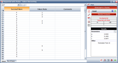
The next figure shows the entered data and the estimated parameters.

Entered data and the estimated Standard Gompertz parameters.

The Gompertz reliability growth curve may now be written as follows where [math]\displaystyle{ {{L}_{G}} }[/math] is the number of launches with the first successful launch being counted as [math]\displaystyle{ {{L}_{G}}=1 }[/math] . Therefore, [math]\displaystyle{ {{L}_{G}} }[/math] is equal to 19, since reliability growth starts with launch 4.

[math]\displaystyle{ R=0.9299{{(0.0943)}^{{{0.7170}^{{{L}_{G}}}}}} }[/math]

2) The predicted reliability after launch 22 is:

[math]\displaystyle{ \begin{align} & R= & 0.9299{{(0.0943)}^{{{0.7170}^{19}}}} \\ & = & 0.9260 \end{align} }[/math]

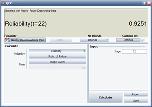
The predicted reliability after launch 22 is calculated using the Quick Calculation Pad and is shown next.

Predicted reliability after launch 22.

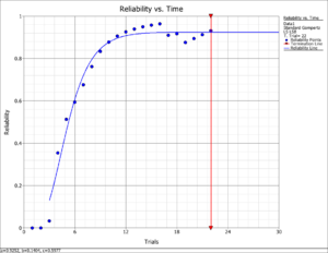
3) In Table A.2, the predicted reliability values are compared with the reliabilities that are calculated from the raw data using failure discounting. It can be seen in the table and in the following figure that the Gompertz curve appears to provide a good fit to the actual data.

Standard Gompertz reliability growth curve.