Event Log Data

Template:LDABOOK SUB Event logs, or maintenance logs, store information about a piece of equipment's failures and repairs. They provide useful information that can help companies achieve their productivity goals by giving insight about the failure modes, frequency of outages, repair duration, uptime/downtime and availability of the equipment. Some event logs contain more information than others, but essentially event logs capture data in a format that includes the type of event, the date/time when the event occurred and the date/time when the system was restored to operation.

The data from event logs can be used to extract failure times and repair times information. Once the times-to-failure data and times-to-repair data have been obtained, a life distribution can be fitted to each data set. The principles and theory for fitting a life distribution is presented in detail in Life Distributions. The process of data extraction and model fitting can be automated using the Weibull++ event log folio.

Converting Event Logs to Failure/Repair Data

For n number of failures and repair actions that took place during the event logging period, the times-to-failure of every unique occurrence of an event are obtained by calculating the time between the last repair and the time the new failure occurred, or:

[math]\displaystyle{ \text{Time-to-Failure}_{i}=t_{i}-r_{i-1}\,\! }[/math]

where:

• [math]\displaystyle{ i=1,...n\,\! }[/math]
• [math]\displaystyle{ t_{i}\,\! }[/math] is the date/time of occurrence of [math]\displaystyle{ i\,\! }[/math].
• [math]\displaystyle{ r_{i-1}\,\! }[/math] is the date/time of restoration of the previous occurrence [math]\displaystyle{ (i-1)\,\! }[/math].

For systems that were new when the collection of the event log data started, the times to first occurrence of every unique event is equivalent to the date/time of the occurrence of the event minus the time the system monitoring started. That is:

[math]\displaystyle{ \text{Time-to-Failure}_{1}=t_{1}-\text{System Start Time}\,\! }[/math]

For systems that were not new when the collection of event log data started, the times to first occurrence of every unique event are considered to be suspensions (right censored) because the system is assumed to have accumulated more hours before the data collection period started (i.e., the time between the start date/time and the first occurrence of an event is not the entire operating time). In this case:

[math]\displaystyle{ \text{Suspension}_{1}=t_{1}-\text{System Start Time}\,\! }[/math]

When monitoring on the system is stopped or when the system is no longer being used, all events that have not occurred by this time are considered to be suspensions.

[math]\displaystyle{ \text{Last Suspension}=\text{System End Time}-r_{n}\,\! }[/math]

The four equations given above are valid for cases in which a component operates through the failure of other components. When the component does not operate through the failures, the assumptions must include the downtime of the system due to the other failures. In other words, the first four equations become:

[math]\displaystyle{ \text{Time-to-Failure}_{i}=t_{i}-r_{i-1}-(\text{System Downtime since}\,r_{i-1})\,\! }[/math]

[math]\displaystyle{ \text{Time-to-Failure}_{1}=t_{1}-(\text{System Start Time}-\text{System Downtime since System Start Time})\,\! }[/math]

[math]\displaystyle{ \text{Suspension}_{1}=t_{1}-(\text{System Start Time}-\text{System Downtime since System Start Time})\,\! }[/math]

[math]\displaystyle{ \text{Last Suspension} = \text{System End Time}-r_{n}-\text{System Downtime since}\,r_{n}\,\! }[/math]

Repair times are obtained by calculating the difference between the date/time of event occurrence and the date/time of restoration, or:

[math]\displaystyle{ \text{Time-to-repair}_{i}=r_{i}-t_{i}\,\! }[/math]

All these equations should also take into consideration the periods when the system is not operating or not in use, as in the case of operations that do not run on a 24/7 basis.

Example: Simple System

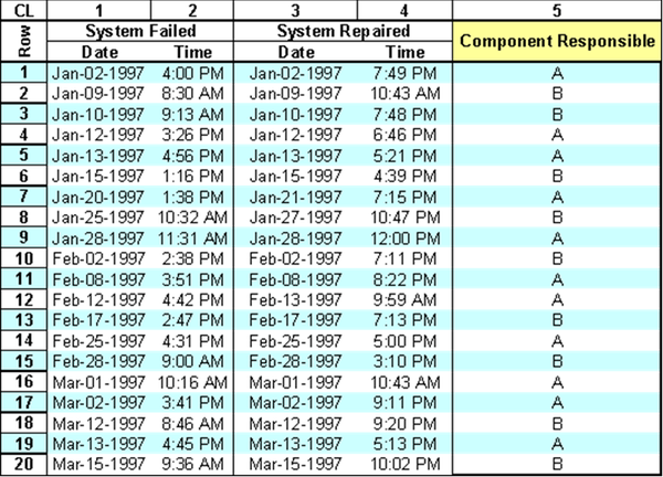
Consider a very simple system composed of only two components, A and B. The system runs from 8 AM to 5 PM, Monday through Friday. When a failure is observed, the system undergoes repair and the failed component is replaced. The date and time of each failure is recorded in an equipment downtime log, along with an indication of the component that caused the failure. The date and time when the system was restored is also recorded. The downtime log for this simple system is given next.

Note that:

• The date and time of each failure is recorded.
• The date and time of repair completion for each failure is recorded.
• The repair involves replacement of the responsible component.
• The responsible component for each failure is recorded.

For this example, we will assume that an engineer began recording these events on January 1, 1997 at 12 PM and stopped recording on March 18, 1997 at 1 PM, at which time the analysis was performed. Information for events prior to January 1 is unknown. The objective of the analysis is to obtain the failure and repair distributions for each component.

Solution

We begin the analysis by looking at component A. The first time that component A is known to have failed is recorded in row 1 of the data sheet; thus, the first age (or time-to-failure) for A is the difference between the time we began recording the data and the time when this failure event happened. Also, the component does not age when the system is down due to the failure of another component. Therefore, this time must be taken into account.

1. The First Time-To-Failure for Component A, TTF_A[1]

The first time-to-failure of component A, TTF_A[1], is the sum of the hours of operation for each day, starting on the start date (and time) and ending with the failure date (and time). This is graphically shown next. The boxes with the green background indicate the operating periods. Thus, TTF_A[1] = 5 + 8 = 13 hours.

2. The First Time-To-Repair for Component A, TTR_A[1]

The time-to-repair for component A for this failure, TTR_A[1], is [Date/Time Restored - Date/Time Occurred] or:

TTR_A[1] = (Jan 02 1997/7:49 PM) - (Jan 02 1997/4:00 PM) = 3:49 = 3.8166 hours

(Note that in the case of repair actions, shifts are not taken into account since it is assumed that repair actions will be performed as needed to bring the system up.)

3. The Second Time-To-Failure for Component A, TTF_A[2]

Continuing with component A, the second system failure due to component A is found in row 4, on January 12, 1997 at 3:26 PM. Thus, to compute TTF_A[2], you must look at the age the component accumulated from the last repair time, taking shifts into account as before, but with the added complexity of accounting for the times that the system was down due to failures of other components (i.e., component A was not aging when the system was down for repair due to a component B failure).

This is graphically shown next using green to show the operating times of A and orange to show the downtimes of the system for reasons other than the failure of A (to the closest hour).

To illustrate this mathematically, we will use a function, [math]\displaystyle{ \tau }[/math], which, given a range of times, returns the shift hours worked during that period. In other words, for this example [math]\displaystyle{ \tau }[/math](1/1/97 3:00 AM - 1/1/97 6:00 PM) = 9 hours given an 8 AM to 5 PM shift. Furthermore, we will show the date and time a failure occurred as DTO and the date and time a repair was completed at DTR with a numerical subscript indicating the row that this entry is in (e.g., DTO₄ for the date and time a failure occurred in row 4).

Then the total possible hours (TPH) that component A could have operated from the time it was repaired to the time it failed the second time is:

TPH = [math]\displaystyle{ \tau }[/math](DTO₄ – DTR₁),

TPH = [math]\displaystyle{ \tau }[/math](DTO₄ – DTR₁) = 9 Days * 9 hours + 7:26 hours = 88:26 hours = 88.433 hours

The time that component A was not operating (NOP) during normal hours of operation is the time that the system was down due to failure of component B, or:

NOP = [math]\displaystyle{ \tau }[/math](DTO₂ – DTR₂) + [math]\displaystyle{ \tau }[/math](DTO₃ – DTR₃)

NOP = [math]\displaystyle{ \tau }[/math](DTO₂ – DTR₂) + [math]\displaystyle{ \tau }[/math]( DTO₃ – DTR₃) = 2:13 hours + 7:47 hours = 10:00 hours

Thus, the second time-to-failure for component A, TTF_A[2], is:

TTF_A [2] = TPH - NOP

TTF_A[2] = 88:26 hours – 10:00 hours = 78:26 hours = 78.433 hours

4. The Second Time-To-Repair for Component A, TTR_A[2]

To compute the time-to-repair for this failure:

TTR_A[2] = [math]\displaystyle{ \tau }[/math] (DTO₄ – DTR₄) = (3 h, 49 m) = 3.8166 hours

5. Computing the Rest of the Observed Failures

This same process can be repeated for the rest of the observed failures, yielding:

TTF_A[3] = 8.9333

TTF_A[4] = 56.25

TTF_A[5] = 33.05

TTF_A[6] = 100.8433

TTF_A[7] = 35.7

TTF_A[8] = 112.3166

TTF_A[9] = 23.1

TTF_A[10] = 13.9666

TTF_A[11] = 90.5166

and

TTR_A[3] = 0.4166

TTR_A[4] = 29.6166

TTR_A[5] = 0.4833

TTR_A[6] = 4.5166

TTR_A[7] = 17.2833

TTR_A[8] = 0.4833

TTR_A[9] = 0.45

TTR_A[10] = 5.5

TTR_A[11] = 0.4666

6. Creating the Data Sets

When the computations shown above are complete, we can create the data set needed to obtain the life distributions for the failure and repair times for component A. To accomplish this, modifications will need to be performed on the TTF data, given the original assumptions, as follows:

• TTF_A[2] through TTF_A[11] will remain as is and be designated as times-to-failure (F).
• TTF_A[1] will be designated as a right censored data point (or suspension, S). This is because when we started collecting data, component A was operating for an unknown period of time X, so the true time-to-failure for component A is the operating time observed (in this case, TTF_A[1] = 13 hours) plus the unknown operating time X. Thus, what we know is that the true time-to-failure for A is some time greater than the observed TTF_A[1] (i.e., a right censored data point).
• An additional right censored observation (suspension) will be added to the data set to reflect the time that component A operated without failure from its last repair time to the end of the observation period. This is presented next.

Since our analysis time ends on March 18, 1997 at 1:00 PM and component A has operated successfully from the last time it was replaced on March 13, 1997 at 5:13 PM, the additional time of successful operation is:

TPH = [math]\displaystyle{ \tau }[/math](End Time – DTR₁₉) = (4 days * 9 hours/day + 5:00 hours) = 41:00 hours

NOP = [math]\displaystyle{ \tau }[/math]( DTO₂₀ – DTR₂₀) = 7:24 hours

Thus, the remaining time that component A operated without failure is:

TTS = TPH - NOP = 33:36 = 33.6 hours.

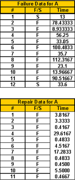
The next two tables show component A's failure and repair data. The entire analysis can be repeated to obtain the failure and repair times for component B.

7. Automated Analysis in Weibull++8

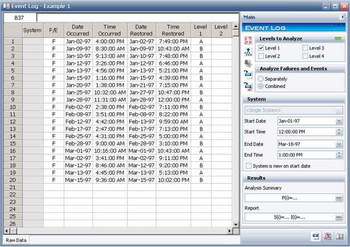
The analysis can be automatically performed in the Weibull++ 8 event log folio. Simply enter the data from the equipment downtime log into the folio, as shown next.

Use the Shift Pattern window (Event Log > Action and Settings > Set Shift Pattern) to specify the 8:00 AM to 5:00 PM shifts that occur seven days a week, as shown next.

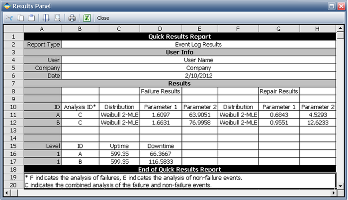
The folio will automatically convert the equipment downtime log data to time-to-failure and time-to-repair data and fit failure and repair distributions to the data set. To view the failure and repair results, click the Show Analysis Summary (...) button on the control panel. The Results window shows the calculated values.

Example: System with Failure and Non-Failure Events

This example is similar to the previous example; however, we will now classify each occurrence as a failure or event, thus adding another level of complexity to the analysis.

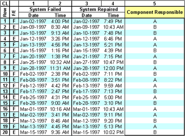
Consider the same data set from the previous example, but with the addition of a column indicating whether the occurrence was a failure (F) or an event (E). (A general event represents an activity that brings the system down but is not directly relevant to the reliability of the equipment, such as preventive maintenance, routine inspections and the like.)

Allowing for the inclusion of an F/E identifier increases the number of items that we will be considering. In other words, the objective now will be to determine a failure and repair distribution for component A due to failure, component B due to failure, component A due to an event and component B due to an event. This is mathematically equivalent to increasing the number of components from two (A and B) to four (FA, EA, FB and EB); thus, the analysis steps are identical to the ones performed in the first example, but for four components instead of two.

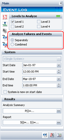
In the Weibull++8 event log folio, to consider the F/E in the analysis, the setting in the Analyze Failures and Events area of the control panel must be set to Separately. Selecting the Combined option will result in ignoring the F and E distinction and treating all entries as Fs (i.e., perform the same analysis as in the first example).

Example: System with Components Operating Through System Failures

We will repeat the first example, but with an interesting twist. In the first example, the assumption was that when the system was down due to a failure, none of the components aged. We will now allow some of these components to age even when the system is down.

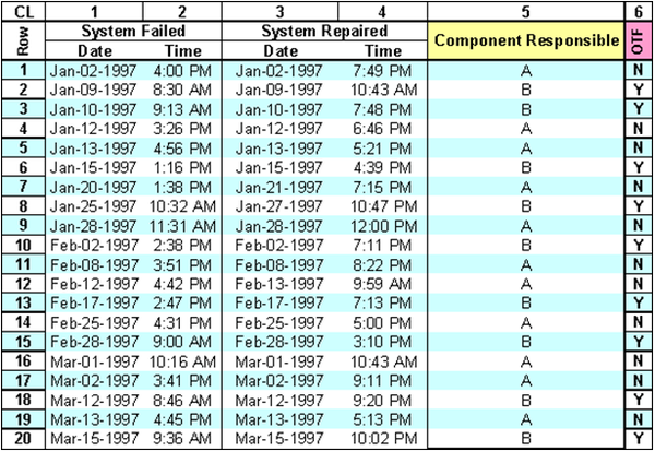
Using the same data as in the first example, we will assume that component B accumulates age when the system is down for any reason other than the failure of component B. Component A will not accumulate age when the system is down. We indicate this in the data sheet in the OTF (Operate Through other Failures) column, where Y = yes and N = no. Note that this entry must be consistent with all other events in the data set associated with the component (i.e., all component A records must show N and all component B records must show Y).

Because component A does not operate through other failures, the analysis steps (and results) are identical to the ones in the first example. However, the analysis for the times-to-failure for component B will be different (and is actually less cumbersome than in the first example because we do not need to subtract the time that the system was down due to the failure of other components).

Specifically:

TTF_B[1] = [math]\displaystyle{ \tau }[/math](Start Time - DTO₂ ) = 68:30 = 68.5 hours

TTF_B[2] = [math]\displaystyle{ \tau }[/math](DTR₂ - DTO₃) = 7:30 = 7.5 hours

TTF_B[3] = [math]\displaystyle{ \tau }[/math](DTR₃ - DTO₆) = 41.26 hours

The TTR analysis is not affected by this setting and is identical to the result in the first example.

Example: System with Sub-Components

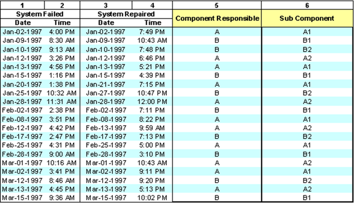
In this example, we will repeat the first example, but use two component levels instead of a single level. Using the same data as in the first example, we will assume that component A has two sub-components, A1 and A2; and component B also has two sub-components, B1 and B2, as shown in the following table.

Analyzing the data for only level 1 will ignore all entries for level 2. However, if performing a level 2 analysis, both entries in level 1 and 2 are taken into account, creating a unique item. More specifically, the analysis for level 2 will be done at the sub-component level and depend on the component that the sub-component belongs to. Note that this is equivalent to reducing the analysis to a single level but looking at each component and sub-component combination individually through the process. In other words, for level 2 analyses, the data set shown above can be reduced to a single level analysis for four items: A-A1, A-A2, B-B1 and B-B2.

This component and sub-component combination will yield a unique item that must be treated separately, much as components A and B were in the first example. The same concept applies when more levels are present. When specifying OTF (Operate Through other Failures) characteristics at this level, each component and sub-component combination is treated differently. In other words, it is possible that A-A1 and A-A2 have different OTF designations, even though they belong to the same component; however, all A-A2s must have the same OTF designation.

---

More event log folio examples are available! See also:

Factory Equipment Failure Log or Watch the video...

---