Electronic Components Example: Difference between revisions
Kate Racaza (talk | contribs) No edit summary |
Chris Kahn (talk | contribs) No edit summary |
||
| Line 1: | Line 1: | ||
<noinclude>{{Banner_ALTA_Examples}}</noinclude> | <noinclude>{{Banner_ALTA_Examples}}</noinclude> | ||
An electronic component was redesigned and then tested to failure at three different temperatures. Six units were tested at each temperature level. At the | An electronic component was redesigned and then tested to failure at three different temperatures. Six units were tested at each temperature level. At the 406 K stress level, however, a unit was removed from the test due to a test equipment failure which led to a failure of the component. A warranty time of one year is to be given, with an expected return of 10% of the population. The following table shows the times-to-failure and test temperatures. | ||
| Line 7: | Line 7: | ||
The operating temperature is | The operating temperature is 356 K. Using the Arrhenius-Weibull model, determine the following: | ||
1) Should the first failure at | 1) Should the first failure at 406 K be included in the analysis? | ||
2) Determine the warranty time for a 90% reliability. | 2) Determine the warranty time for a 90% reliability. | ||
| Line 27: | Line 27: | ||
1) Since the failure occurred at the very beginning of the test and for an unrelated reason, it can be omitted from the analysis. If it is included it should be treated as a suspension and not as a failure. | 1) Since the failure occurred at the very beginning of the test and for an unrelated reason, it can be omitted from the analysis. If it is included it should be treated as a suspension and not as a failure. | ||
2) Disregard the first failure at | 2) Disregard the first failure at 406 K and analyze the data using the ALTA standard folio. The estimated parameters are: | ||
| Line 57: | Line 57: | ||
A more accurate way to determine the warranty time would be to use ALTA's Quick Calculation Pad (QCP) | A more accurate way to determine the warranty time would be to use ALTA's Quick Calculation Pad (QCP), which estimates the reliable life to be 11,977.792719 hours, as shown next: | ||
| Line 63: | Line 63: | ||
3) From the use level probability plot, the warranty time for a 90% reliability was estimated to be approximately 12,000 | 3) From the use level probability plot, the warranty time for a 90% reliability was estimated to be approximately 12,000 hours. This is above the 1 year (8,760 hours) requirement. However, this is an estimate at the 50% confidence level. In other words, 50% of the time life will be greater than 12,000 hours and 50% of the time life will be less. A known confidence level is therefore crucial before any decisions are made. | ||
Plot the confidence bounds on both probability and Arrhenius plots. The following use level probability plot, shows the 90% lower confidence level (LCL). Note that in ALTA, percentile bounds are Type 1 confidence bounds. | Plot the confidence bounds on both probability and Arrhenius plots. The following use level probability plot, shows the 90% lower confidence level (LCL). Note that in ALTA, percentile bounds are Type 1 confidence bounds. | ||
| Line 77: | Line 77: | ||
You can use the QCP to calculate calculate the lower confidence bound. The result shows a lower bound of 4,436.506367 hours. | |||
| Line 83: | Line 83: | ||
4) The warranty time for this component is estimated to be 4,436.5 | 4) The warranty time for this component is estimated to be 4,436.5 hours at a 90% lower confidence bound. This is much less than the 1 year warranty time required (almost 6 months). Thus the desired warranty is not met. In this case, the following four options are available: | ||
:a) Redesign. | :a) Redesign. | ||
| Line 93: | Line 93: | ||
:d) Test additional units at stress levels closer to the use level. | :d) Test additional units at stress levels closer to the use level. | ||
5) Including the unrelated failure of 0.3 | 5) Including the unrelated failure of 0.3 hours at 406 K (by treating it as a suspension) in the analysis obtains the following results: | ||
| Line 122: | Line 122: | ||
6) Repeat the analysis treating the unrelated failure at 500 | 6) Repeat the analysis treating the unrelated failure at 500 hours as a suspension. The results are: | ||
| Line 145: | Line 145: | ||
As you can see, it would be a mistake to neglect the unrelated failure in this case. By neglecting this failure, we would actually underestimate the warranty time. The important observation in this example is that every piece of life information is crucial. In other words, unrelated failures also provide information about the life of the product. An unrelated failure occurring at 500 | As you can see, it would be a mistake to neglect the unrelated failure in this case. By neglecting this failure, we would actually underestimate the warranty time. The important observation in this example is that every piece of life information is crucial. In other words, unrelated failures also provide information about the life of the product. An unrelated failure occurring at 500 hours indicates that the product has survived for that period of time under the particular stress level; thus, neglecting it would be a mistake. On the other hand, it would also be a mistake to treat this data point as a failure, since the failure was caused by the faulty test equipment. | ||
Latest revision as of 08:04, 15 August 2012
New format available! This reference is now available in a new format that offers faster page load, improved display for calculations and images and more targeted search.
As of January 2024, this Reliawiki page will not continue to be updated. Please update all links and bookmarks to the latest references at ALTA examples and ALTA reference examples.
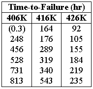
An electronic component was redesigned and then tested to failure at three different temperatures. Six units were tested at each temperature level. At the 406 K stress level, however, a unit was removed from the test due to a test equipment failure which led to a failure of the component. A warranty time of one year is to be given, with an expected return of 10% of the population. The following table shows the times-to-failure and test temperatures.
The operating temperature is 356 K. Using the Arrhenius-Weibull model, determine the following:
1) Should the first failure at 406 K be included in the analysis?
2) Determine the warranty time for a 90% reliability.
3) Determine the 90% lower confidence limit on the warranty time.
4) Is the warranty requirement met? If not, what steps should be taken?
5) Repeat the analysis with the unrelated failure included. Is there any difference?
6) If the unrelated failure occurred at 500 hr, should it be included in the analysis?
Solution
1) Since the failure occurred at the very beginning of the test and for an unrelated reason, it can be omitted from the analysis. If it is included it should be treated as a suspension and not as a failure.
2) Disregard the first failure at 406 K and analyze the data using the ALTA standard folio. The estimated parameters are:
- [math]\displaystyle{ \begin{align} \beta =\ & 2.965820 \\ B=\ & 10679.567542 \\ C=\ & 2.396615\cdot {{10}^{-9}} \end{align} }[/math]
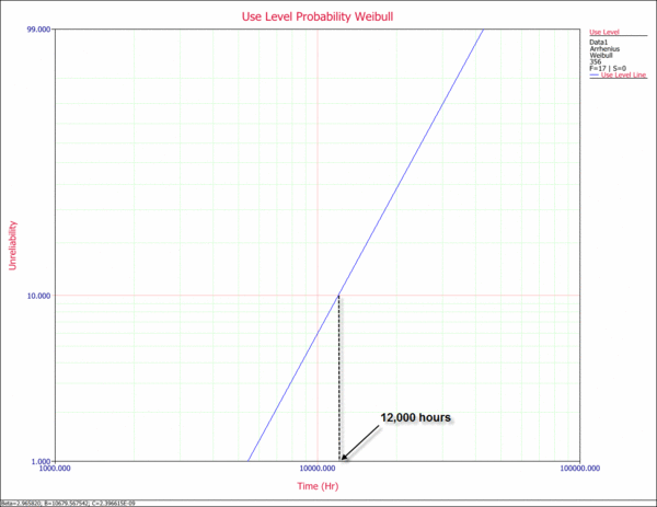
The following plot shows the use level probability plot of the analysis. The warranty time for a reliability of 90% (or an unreliability of 10%) can be estimated from this plot, as shown next.
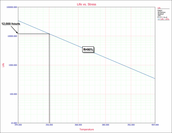
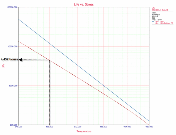
This estimate can also be obtained from the Arrhenius plot (Life vs. Stress plot). The 10th percentile (time for a reliability of 90%) is plotted versus stress. This type of plot is useful because it allows you to determine a time for a given reliability for different stress levels.
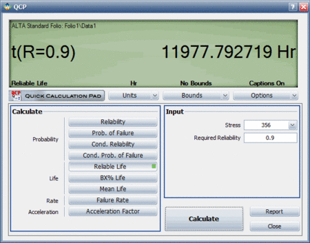
A more accurate way to determine the warranty time would be to use ALTA's Quick Calculation Pad (QCP), which estimates the reliable life to be 11,977.792719 hours, as shown next:
3) From the use level probability plot, the warranty time for a 90% reliability was estimated to be approximately 12,000 hours. This is above the 1 year (8,760 hours) requirement. However, this is an estimate at the 50% confidence level. In other words, 50% of the time life will be greater than 12,000 hours and 50% of the time life will be less. A known confidence level is therefore crucial before any decisions are made.
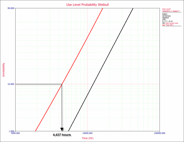
Plot the confidence bounds on both probability and Arrhenius plots. The following use level probability plot, shows the 90% lower confidence level (LCL). Note that in ALTA, percentile bounds are Type 1 confidence bounds.
From the plot, we obtain an estimate of 4,437 hr warranty time at a 90% lower confidence level. This means that 90% of the time, life will be greater than this value. In other words, a life of 4,437 hr is a bounding value for the warranty. The Arrhenius plot with the 90% lower confidence level is shown next.
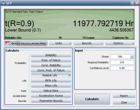
You can use the QCP to calculate calculate the lower confidence bound. The result shows a lower bound of 4,436.506367 hours.
4) The warranty time for this component is estimated to be 4,436.5 hours at a 90% lower confidence bound. This is much less than the 1 year warranty time required (almost 6 months). Thus the desired warranty is not met. In this case, the following four options are available:
- a) Redesign.
- b) Reduce the confidence level.
- c) Change the warranty policy.
- d) Test additional units at stress levels closer to the use level.
5) Including the unrelated failure of 0.3 hours at 406 K (by treating it as a suspension) in the analysis obtains the following results:
- [math]\displaystyle{ \begin{align} \beta =\ & 2.965804 \\ B=\ & 10679.566625 \\ C=\ & 2.396619\cdot {{10}^{-9}} \end{align} }[/math]
These results are essentially identical to the results obtained when the unrelated failure was excluded. A small difference can be seen only if more significant digits are considered. The warranty time with the 90% lower 1-sided confidence bound is estimated to be:
- [math]\displaystyle{ \begin{align} T=\ & 11977.729145\text{ hr} \\ {{T}_{L}}=\ & 4436.462084\text{ hr} \end{align} }[/math]
Again, the difference is negligible. This is due to the very early time at which this unrelated failure occurred.
6) Repeat the analysis treating the unrelated failure at 500 hours as a suspension. The results are:
- [math]\displaystyle{ \begin{align} \beta =\ & 3.022714 \\ B=\ & 10959.523204 \\ C=\ & 1.23808\cdot {{10}^{-9}} \end{align} }[/math]
In this case, the results are very different. The warranty time with the 90% lower 1-sided confidence bound is estimated to be:
- [math]\displaystyle{ \begin{align} T=\ & 13780.208409\text{ hr} \\ {{T}_{L}}=\ & 5303.672050\text{ hr} \end{align} }[/math]
As you can see, it would be a mistake to neglect the unrelated failure in this case. By neglecting this failure, we would actually underestimate the warranty time. The important observation in this example is that every piece of life information is crucial. In other words, unrelated failures also provide information about the life of the product. An unrelated failure occurring at 500 hours indicates that the product has survived for that period of time under the particular stress level; thus, neglecting it would be a mistake. On the other hand, it would also be a mistake to treat this data point as a failure, since the failure was caused by the faulty test equipment.

