Template:Example: Lognormal Distribution RRY: Difference between revisions
No edit summary |
No edit summary |
||
| Line 3: | Line 3: | ||
Fourteen units were reliability tested and the following life test data were obtained: | Fourteen units were reliability tested and the following life test data were obtained: | ||
{|align="center" border= | {|border="1" align="center" style="border-collapse: collapse;" cellpadding="5" cellspacing="5" | ||
|- | |- | ||
|colspan="2" style="text-align:center"| Table 1 - Life Test Data | |colspan="2" style="text-align:center"| Table 1 - Life Test Data | ||
| Line 66: | Line 66: | ||
\end{matrix}</math></center> | \end{matrix}</math></center> | ||
The median rank values ( <math>F({{t}_{i}})</math> ) can be found in rank tables or by using the Quick Statistical Reference in Weibull++ . | The median rank values ( <math>F({{t}_{i}})</math> ) can be found in rank tables or by using the Quick Statistical Reference in Weibull++ . | ||
| Line 73: | Line 72: | ||
Given the values in the table above, calculate <math>\widehat{a}</math> and <math>\widehat{b}</math>: | Given the values in the table above, calculate <math>\widehat{a}</math> and <math>\widehat{b}</math>: | ||
::<math>\begin{align} | ::<math>\begin{align} | ||
| Line 119: | Line 117: | ||
The above example can be repeated using Weibull++ , using RRY. | The above example can be repeated using Weibull++ , using RRY. | ||
[[Image:Lognormal Distribution Example 2 Data and Result.png | [[Image:Lognormal Distribution Example 2 Data and Result.png|center|550px| ]] | ||
The mean can be obtained from the QCP and both the mean and the standard deviation can be obtained from the Function Wizard. | The mean can be obtained from the QCP and both the mean and the standard deviation can be obtained from the Function Wizard. | ||
Revision as of 04:58, 8 August 2012
Lognormal Distribution RRY Example
Fourteen units were reliability tested and the following life test data were obtained:
| Table 1 - Life Test Data | |
| Data point index | Time-to-failure |
|---|---|
| 1 | 5 |
| 2 | 10 |
| 3 | 15 |
| 4 | 20 |
| 5 | 25 |
| 6 | 30 |
| 7 | 35 |
| 8 | 40 |
| 9 | 50 |
| 10 | 60 |
| 11 | 70 |
| 12 | 80 |
| 13 | 90 |
| 14 | 100 |
Assuming the data follow a lognormal distribution, estimate the parameters and the correlation coefficient, [math]\displaystyle{ \rho }[/math] , using rank regression on Y.
Solution
Construct Table 2, as shown next.
The median rank values ( [math]\displaystyle{ F({{t}_{i}}) }[/math] ) can be found in rank tables or by using the Quick Statistical Reference in Weibull++ .
The [math]\displaystyle{ {{y}_{i}} }[/math] values were obtained from the standardized normal distribution's area tables by entering for [math]\displaystyle{ F(z) }[/math] and getting the corresponding [math]\displaystyle{ z }[/math] value ( [math]\displaystyle{ {{y}_{i}} }[/math] ).
Given the values in the table above, calculate [math]\displaystyle{ \widehat{a} }[/math] and [math]\displaystyle{ \widehat{b} }[/math]:
- [math]\displaystyle{ \begin{align} & \widehat{b}= & \frac{\underset{i=1}{\overset{14}{\mathop{\sum }}}\,t_{i}^{\prime }{{y}_{i}}-(\underset{i=1}{\overset{14}{\mathop{\sum }}}\,t_{i}^{\prime })(\underset{i=1}{\overset{14}{\mathop{\sum }}}\,{{y}_{i}})/14}{\underset{i=1}{\overset{14}{\mathop{\sum }}}\,t_{i}^{\prime 2}-{{(\underset{i=1}{\overset{14}{\mathop{\sum }}}\,t_{i}^{\prime })}^{2}}/14} \\ & & \\ & \widehat{b}= & \frac{10.4473-(49.2220)(0)/14}{183.1530-{{(49.2220)}^{2}}/14} \end{align} }[/math]
or:
- [math]\displaystyle{ \widehat{b}=1.0349 }[/math]
and:
- [math]\displaystyle{ \widehat{a}=\frac{\underset{i=1}{\overset{N}{\mathop{\sum }}}\,{{y}_{i}}}{N}-\widehat{b}\frac{\underset{i=1}{\overset{N}{\mathop{\sum }}}\,t_{i}^{\prime }}{N} }[/math]
or:
- [math]\displaystyle{ \widehat{a}=\frac{0}{14}-(1.0349)\frac{49.2220}{14}=-3.6386 }[/math]
- Therefore:
- [math]\displaystyle{ {\sigma'}=\frac{1}{\widehat{b}}=\frac{1}{1.0349}=0.9663 }[/math]
and:
- [math]\displaystyle{ {\mu }'=-\widehat{a}\cdot {\sigma'}=-(-3.6386)\cdot 0.9663 }[/math]
or:
- [math]\displaystyle{ {\mu }'=3.516 }[/math]
The mean and the standard deviation of the lognormal distribution are obtained using equations in section Lognormal Statistical Properties:
- [math]\displaystyle{ \overline{T}=\mu ={{e}^{3.516+\tfrac{1}{2}{{0.9663}^{2}}}}=53.6707\text{ hours} }[/math]
and:
- [math]\displaystyle{ {\sigma}=\sqrt{({{e}^{2\cdot 3.516+{{0.9663}^{2}}}})({{e}^{{{0.9663}^{2}}}}-1)}=66.69\text{ hours} }[/math]
The correlation coefficient can be estimated as:
- [math]\displaystyle{ \widehat{\rho }=0.9754 }[/math]
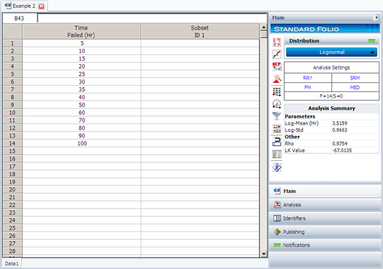
The above example can be repeated using Weibull++ , using RRY.
The mean can be obtained from the QCP and both the mean and the standard deviation can be obtained from the Function Wizard.
