Template:Example: Lognormal Distribution RRX

Lognormal Distribution RRX Example

Using the data of Example 2 and assuming a lognormal distribution, estimate the parameters and estimate the correlation coefficient, [math]\displaystyle{ \rho }[/math] , using rank regression on X.

Solution

Table 2 constructed in Example 2 applies to this example as well. Using the values in this table we get:

[math]\displaystyle{ \begin{align} & \hat{b}= & \frac{\underset{i=1}{\overset{14}{\mathop{\sum }}}\,t_{i}^{\prime }{{y}_{i}}-\tfrac{\underset{i=1}{\overset{14}{\mathop{\sum }}}\,t_{i}^{\prime }\underset{i=1}{\overset{14}{\mathop{\sum }}}\,{{y}_{i}}}{14}}{\underset{i=1}{\overset{14}{\mathop{\sum }}}\,y_{i}^{2}-\tfrac{{{\left( \underset{i=1}{\overset{14}{\mathop{\sum }}}\,{{y}_{i}} \right)}^{2}}}{14}} \\ & & \\ & \widehat{b}= & \frac{10.4473-(49.2220)(0)/14}{11.3646-{{(0)}^{2}}/14} \end{align} }[/math]

or:

[math]\displaystyle{ \widehat{b}=0.9193 }[/math]

and:

[math]\displaystyle{ \hat{a}=\overline{x}-\hat{b}\overline{y}=\frac{\underset{i=1}{\overset{14}{\mathop{\sum }}}\,t_{i}^{\prime }}{14}-\widehat{b}\frac{\underset{i=1}{\overset{14}{\mathop{\sum }}}\,{{y}_{i}}}{14} }[/math]

or:

[math]\displaystyle{ \widehat{a}=\frac{49.2220}{14}-(0.9193)\frac{(0)}{14}=3.5159 }[/math]

Therefore:

[math]\displaystyle{ {\sigma'}=\widehat{b}=0.9193 }[/math]

and:

[math]\displaystyle{ {\mu }'=\frac{\widehat{a}}{\widehat{b}}{\sigma'}=\frac{3.5159}{0.9193}\cdot 0.9193=3.5159 }[/math]

Using for Mean and Standard Deviation we get:

[math]\displaystyle{ \overline{T}=\mu =51.3393\text{ hours} }[/math]

and:

[math]\displaystyle{ {\sigma'}=59.1682\text{ hours}. }[/math]

The correlation coefficient is found using the equation in previous section:

[math]\displaystyle{ \widehat{\rho }=0.9754. }[/math]

Note that the regression on Y analysis is not necessarily the same as the regression on X. The only time when the results of the two regression types are the same (i.e., will yield the same equation for a line) is when the data lie perfectly on a line.

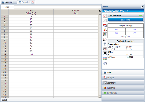
Using Weibull++ , with the Rank Regression on X option, the results are: