Distributions Used in Accelerated Testing

In this chapter, we will briefly present three lifetime distributions commonly used in accelerated life test analysis: the 1-parameter exponential, the 2-parameter Weibull and the lognormal distributions. Readers who are interested in a more rigorous overview (or in different forms of these and other life distributions) can refer to ReliaSoft's Life Data Analysis Reference. For information about the parameter estimation methods, see Appendix B.

The Exponential Distribution

The exponential distribution is a very commonly used distribution in reliability engineering. Due to its simplicity, it has been widely employed, even in cases where it doesn't apply. The exponential distribution is used to describe units that have a constant failure rate. The 1-parameter exponential pdf is given by:

[math]\displaystyle{ \begin{align} & f(T)= \lambda {{e}^{-\lambda T}}=\frac{1}{m}{{e}^{-\tfrac{1}{m}T}} \\ & T\ge 0,\lambda \gt 0,m\gt 0 \end{align} }[/math]

where:

• λ = constant failure rate, in failures per unit of measurement (e.g. failures per hour, per cycle, etc.).
• [math]\displaystyle{ \lambda =\tfrac{1}{m} }[/math].
• m = mean time between failures, or to a failure.
• T = operating time, life, or age, in hours, cycles, miles, actuations, etc. This distribution requires the estimation of only one parameter, λ , for its application.

Exponential Distribution Functions

The Mean or MTTF

The mean, [math]\displaystyle{ \overline{T},\,\! }[/math] or mean time to failure (MTTF) is given by:

[math]\displaystyle{ \begin{align} \bar{T}= & \int_{\gamma }^{\infty }t\cdot f(t)dt \\ = & \int_{\gamma }^{\infty }t\cdot \lambda \cdot {{e}^{-\lambda t}}dt \\ = & \gamma +\frac{1}{\lambda }=m \end{align}\,\! }[/math]

Note that when [math]\displaystyle{ \gamma =0\,\! }[/math], the MTTF is the inverse of the exponential distribution's constant failure rate. This is only true for the exponential distribution. Most other distributions do not have a constant failure rate. Consequently, the inverse relationship between failure rate and MTTF does not hold for these other distributions.

The Median

The median, [math]\displaystyle{ \breve{T}, \,\! }[/math] is:

[math]\displaystyle{ \breve{T}=\gamma +\frac{1}{\lambda}\cdot 0.693 \,\! }[/math]

The Mode

The mode, [math]\displaystyle{ \tilde{T},\,\! }[/math] is:

[math]\displaystyle{ \tilde{T}=\gamma \,\! }[/math]

The Standard Deviation

The standard deviation, [math]\displaystyle{ {\sigma }_{T}\,\! }[/math], is:

[math]\displaystyle{ {\sigma}_{T}=\frac{1}{\lambda }=m\,\! }[/math]

The Exponential Reliability Function

The equation for the 2-parameter exponential cumulative density function, or cdf, is given by:

[math]\displaystyle{ \begin{align} F(t)=Q(t)=1-{{e}^{-\lambda (t-\gamma )}} \end{align}\,\! }[/math]

Recalling that the reliability function of a distribution is simply one minus the cdf, the reliability function of the 2-parameter exponential distribution is given by:

[math]\displaystyle{ R(t)=1-Q(t)=1-\int_{0}^{t-\gamma }f(x)dx\,\! }[/math]

[math]\displaystyle{ R(t)=1-\int_{0}^{t-\gamma }\lambda {{e}^{-\lambda x}}dx={{e}^{-\lambda (t-\gamma )}}\,\! }[/math]

The 1-parameter exponential reliability function is given by:

[math]\displaystyle{ R(t)={{e}^{-\lambda t}}={{e}^{-\tfrac{t}{m}}}\,\! }[/math]

The Exponential Conditional Reliability Function

The exponential conditional reliability equation gives the reliability for a mission of [math]\displaystyle{ t\,\! }[/math] duration, having already successfully accumulated [math]\displaystyle{ T\,\! }[/math] hours of operation up to the start of this new mission. The exponential conditional reliability function is:

[math]\displaystyle{ R(t|T)=\frac{R(T+t)}{R(T)}=\frac{{{e}^{-\lambda (T+t-\gamma )}}}{{{e}^{-\lambda (T-\gamma )}}}={{e}^{-\lambda t}}\,\! }[/math]

which says that the reliability for a mission of [math]\displaystyle{ t\,\! }[/math] duration undertaken after the component or equipment has already accumulated [math]\displaystyle{ T\,\! }[/math] hours of operation from age zero is only a function of the mission duration, and not a function of the age at the beginning of the mission. This is referred to as the memoryless property.

The Exponential Reliable Life Function

The reliable life, or the mission duration for a desired reliability goal, [math]\displaystyle{ {{t}_{R}}\,\! }[/math], for the 1-parameter exponential distribution is:

[math]\displaystyle{ R({{t}_{R}})={{e}^{-\lambda ({{t}_{R}}-\gamma )}}\,\! }[/math]

[math]\displaystyle{ \begin{align} \ln[R({{t}_{R}})]=-\lambda({{t}_{R}}-\gamma ) \end{align}\,\! }[/math]

or:

[math]\displaystyle{ {{t}_{R}}=\gamma -\frac{\ln [R({{t}_{R}})]}{\lambda }\,\! }[/math]

The Exponential Failure Rate Function

The exponential failure rate function is:

[math]\displaystyle{ \lambda (t)=\frac{f(t)}{R(t)}=\frac{\lambda {{e}^{-\lambda (t-\gamma )}}}{{{e}^{-\lambda (t-\gamma )}}}=\lambda =\text{constant}\,\! }[/math]

Once again, note that the constant failure rate is a characteristic of the exponential distribution, and special cases of other distributions only. Most other distributions have failure rates that are functions of time.

Characteristics of the Exponential Distribution

The primary trait of the exponential distribution is that it is used for modeling the behavior of items with a constant failure rate. It has a fairly simple mathematical form, which makes it fairly easy to manipulate. Unfortunately, this fact also leads to the use of this model in situations where it is not appropriate. For example, it would not be appropriate to use the exponential distribution to model the reliability of an automobile. The constant failure rate of the exponential distribution would require the assumption that the automobile would be just as likely to experience a breakdown during the first mile as it would during the one-hundred-thousandth mile. Clearly, this is not a valid assumption. However, some inexperienced practitioners of reliability engineering and life data analysis will overlook this fact, lured by the siren-call of the exponential distribution's relatively simple mathematical models.

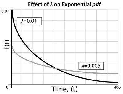
The Effect of lambda and gamma on the Exponential pdf

• The exponential pdf has no shape parameter, as it has only one shape.
• The exponential pdf is always convex and is stretched to the right as [math]\displaystyle{ \lambda \,\! }[/math] decreases in value.
• The value of the pdf function is always equal to the value of [math]\displaystyle{ \lambda \,\! }[/math] at [math]\displaystyle{ t=0\,\! }[/math] (or [math]\displaystyle{ t=\gamma \,\! }[/math]).
• The location parameter, [math]\displaystyle{ \gamma \,\! }[/math], if positive, shifts the beginning of the distribution by a distance of [math]\displaystyle{ \gamma \,\! }[/math] to the right of the origin, signifying that the chance failures start to occur only after [math]\displaystyle{ \gamma \,\! }[/math] hours of operation, and cannot occur before this time.
• The scale parameter is [math]\displaystyle{ \tfrac{1}{\lambda }=\bar{T}-\gamma =m-\gamma \,\! }[/math].
• As [math]\displaystyle{ t\to \infty \,\! }[/math], [math]\displaystyle{ f(t)\to 0\,\! }[/math].

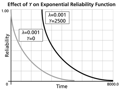
The Effect of lambda and gamma on the Exponential Reliability Function

• The 1-parameter exponential reliability function starts at the value of 100% at [math]\displaystyle{ t=0\,\! }[/math], decreases thereafter monotonically and is convex.
• The 2-parameter exponential reliability function remains at the value of 100% for [math]\displaystyle{ t=0\,\! }[/math] up to [math]\displaystyle{ t=\gamma \,\! }[/math], and decreases thereafter monotonically and is convex.
• As [math]\displaystyle{ t\to \infty \,\! }[/math], [math]\displaystyle{ R(t\to \infty )\to 0\,\! }[/math].
• The reliability for a mission duration of [math]\displaystyle{ t=m=\tfrac{1}{\lambda }\,\! }[/math], or of one MTTF duration, is always equal to [math]\displaystyle{ 0.3679\,\! }[/math] or 36.79%. This means that the reliability for a mission which is as long as one MTTF is relatively low and is not recommended because only 36.8% of the missions will be completed successfully. In other words, of the equipment undertaking such a mission, only 36.8% will survive their mission.

The Effect of lambda and gamma on the Failure Rate Function

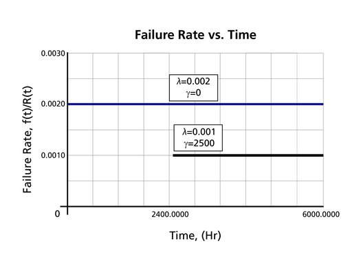
• The 1-parameter exponential failure rate function is constant and starts at [math]\displaystyle{ t=0\,\! }[/math].
• The 2-parameter exponential failure rate function remains at the value of 0 for [math]\displaystyle{ t=0\,\! }[/math] up to [math]\displaystyle{ t=\gamma \,\! }[/math], and then keeps at the constant value of [math]\displaystyle{ \lambda\,\! }[/math].

The Weibull Distribution

The Weibull distribution is a general purpose reliability distribution used to model material strength, times-to-failure of electronic and mechanical components, equipment or systems. In its most general case, the 3-parameter Weibull pdf is defined by:

[math]\displaystyle{ f(t)=\frac{\beta}{\eta } \left( \frac{t-\gamma }{\eta } \right)^{\beta -1}{e}^{-(\tfrac{t-\gamma }{\eta }) ^{\beta}}\,\! }[/math]

where [math]\displaystyle{ \beta \,\! }[/math] = shape parameter, [math]\displaystyle{ \eta \,\! }[/math] = scale parameter and [math]\displaystyle{ \gamma\,\! }[/math] = location parameter.

If the location parameter, [math]\displaystyle{ \gamma\,\! }[/math], is assumed to be zero, then the distribution becomes the 2-parameter Weibull or:

[math]\displaystyle{ f(t)=\frac{\beta}{\eta }( \frac{t }{\eta } )^{\beta -1}{e}^{-(\tfrac{t }{\eta }) ^{\beta}}\,\! }[/math]

One additional form is the 1-parameter Weibull distribution, which assumes that the location parameter, [math]\displaystyle{ \gamma\,\! }[/math] is zero, and the shape parameter is a known constant, or [math]\displaystyle{ \beta \,\! }[/math] = constant = [math]\displaystyle{ C\,\! }[/math], so:

[math]\displaystyle{ f(t)=\frac{C}{\eta}(\frac{t}{\eta})^{C-1}e^{-(\frac{t}{\eta})^C} \,\! }[/math]

For a detailed discussion of this distribution, see The Weibull Distribution.

Weibull Distribution Functions

The Mean or MTTF

The mean, [math]\displaystyle{ \overline{T} \,\! }[/math], (also called MTTF) of the Weibull pdf is given by:

[math]\displaystyle{ \overline{T}=\gamma +\eta \cdot \Gamma \left( {\frac{1}{\beta }}+1\right) \,\! }[/math]

where

[math]\displaystyle{ \Gamma \left( {\frac{1}{\beta }}+1\right) \,\! }[/math]

is the gamma function evaluated at the value of:

[math]\displaystyle{ \left( { \frac{1}{\beta }}+1\right) \,\! }[/math]

The gamma function is defined as:

[math]\displaystyle{ \Gamma (n)=\int_{0}^{\infty }e^{-x}x^{n-1}dx \,\! }[/math]

For the 2-parameter case, this can be reduced to:

[math]\displaystyle{ \overline{T}=\eta \cdot \Gamma \left( {\frac{1}{\beta }}+1\right) \,\! }[/math]

Note that some practitioners erroneously assume that [math]\displaystyle{ \eta \,\! }[/math] is equal to the MTTF, [math]\displaystyle{ \overline{T}\,\! }[/math]. This is only true for the case of: [math]\displaystyle{ \beta=1 \,\! }[/math] or:

[math]\displaystyle{ \begin{align} \overline{T} &= \eta \cdot \Gamma \left( {\frac{1}{1}}+1\right) \\ &= \eta \cdot \Gamma \left( {\frac{1}{1}}+1\right) \\ &= \eta \cdot \Gamma \left( {2}\right) \\ &= \eta \cdot 1\\ &= \eta \end{align} \,\! }[/math]

The Median

The median, [math]\displaystyle{ \breve{T}\,\! }[/math], of the Weibull distribution is given by:

[math]\displaystyle{ \breve{T}=\gamma +\eta \left( \ln 2\right) ^{\frac{1}{\beta }} \,\! }[/math]

The Mode

The mode, [math]\displaystyle{ \tilde{T} \,\! }[/math], is given by:

[math]\displaystyle{ \tilde{T}=\gamma +\eta \left( 1-\frac{1}{\beta }\right) ^{\frac{1}{\beta }} \,\! }[/math]

The Standard Deviation

The standard deviation, [math]\displaystyle{ \sigma _{T}\,\! }[/math], is given by:

[math]\displaystyle{ \sigma _{T}=\eta \cdot \sqrt{\Gamma \left( {\frac{2}{\beta }}+1\right) -\Gamma \left( {\frac{1}{ \beta }}+1\right) ^{2}} \,\! }[/math]

The Weibull Reliability Function

The equation for the 3-parameter Weibull cumulative density function, cdf, is given by:

[math]\displaystyle{ F(t)=1-e^{-\left( \frac{t-\gamma }{\eta }\right) ^{\beta }} \,\! }[/math]

This is also referred to as unreliability and designated as [math]\displaystyle{ Q(t) \,\! }[/math] by some authors.

Recalling that the reliability function of a distribution is simply one minus the cdf, the reliability function for the 3-parameter Weibull distribution is then given by:

[math]\displaystyle{ R(t)=e^{-\left( { \frac{t-\gamma }{\eta }}\right) ^{\beta }} \,\! }[/math]

The Weibull Conditional Reliability Function

The 3-parameter Weibull conditional reliability function is given by:

[math]\displaystyle{ R(t|T)={ \frac{R(T+t)}{R(T)}}={\frac{e^{-\left( {\frac{T+t-\gamma }{\eta }}\right) ^{\beta }}}{e^{-\left( {\frac{T-\gamma }{\eta }}\right) ^{\beta }}}} \,\! }[/math]

or:

[math]\displaystyle{ R(t|T)=e^{-\left[ \left( {\frac{T+t-\gamma }{\eta }}\right) ^{\beta }-\left( {\frac{T-\gamma }{\eta }}\right) ^{\beta }\right] } \,\! }[/math]

These give the reliability for a new mission of [math]\displaystyle{ t \,\! }[/math] duration, having already accumulated [math]\displaystyle{ T \,\! }[/math] time of operation up to the start of this new mission, and the units are checked out to assure that they will start the next mission successfully. It is called conditional because you can calculate the reliability of a new mission based on the fact that the unit or units already accumulated hours of operation successfully.

The Weibull Reliable Life

The reliable life, [math]\displaystyle{ T_{R}\,\! }[/math], of a unit for a specified reliability, [math]\displaystyle{ R\,\! }[/math], starting the mission at age zero, is given by:

[math]\displaystyle{ T_{R}=\gamma +\eta \cdot \left\{ -\ln ( R ) \right\} ^{ \frac{1}{\beta }} \,\! }[/math]

This is the life for which the unit/item will be functioning successfully with a reliability of [math]\displaystyle{ R\,\! }[/math]. If [math]\displaystyle{ R = 0.50\,\! }[/math], then [math]\displaystyle{ T_{R}=\breve{T} \,\! }[/math], the median life, or the life by which half of the units will survive.

The Weibull Failure Rate Function

The Weibull failure rate function, [math]\displaystyle{ \lambda(t) \,\! }[/math], is given by:

[math]\displaystyle{ \lambda \left( t\right) = \frac{f\left( t\right) }{R\left( t\right) }=\frac{\beta }{\eta }\left( \frac{ t-\gamma }{\eta }\right) ^{\beta -1} \,\! }[/math]

Characteristics of the Weibull Distribution

The Weibull distribution is widely used in reliability and life data analysis due to its versatility. Depending on the values of the parameters, the Weibull distribution can be used to model a variety of life behaviors. We will now examine how the values of the shape parameter, [math]\displaystyle{ \beta\,\! }[/math], and the scale parameter, [math]\displaystyle{ \eta\,\! }[/math], affect such distribution characteristics as the shape of the curve, the reliability and the failure rate. Note that in the rest of this section we will assume the most general form of the Weibull distribution, (i.e., the 3-parameter form). The appropriate substitutions to obtain the other forms, such as the 2-parameter form where [math]\displaystyle{ \gamma = 0,\,\! }[/math] or the 1-parameter form where [math]\displaystyle{ \beta = C = \,\! }[/math] constant, can easily be made.

Effects of the Shape Parameter, beta

The Weibull shape parameter, [math]\displaystyle{ \beta\,\! }[/math], is also known as the slope. This is because the value of [math]\displaystyle{ \beta\,\! }[/math] is equal to the slope of the regressed line in a probability plot. Different values of the shape parameter can have marked effects on the behavior of the distribution. In fact, some values of the shape parameter will cause the distribution equations to reduce to those of other distributions. For example, when [math]\displaystyle{ \beta = 1\,\! }[/math], the pdf of the 3-parameter Weibull distribution reduces to that of the 2-parameter exponential distribution or:

[math]\displaystyle{ f(t)={\frac{1}{\eta }}e^{-{\frac{t-\gamma }{\eta }}} \,\! }[/math]

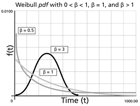
where [math]\displaystyle{ \frac{1}{\eta }=\lambda = \,\! }[/math] failure rate. The parameter [math]\displaystyle{ \beta\,\! }[/math] is a pure number, (i.e., it is dimensionless). The following figure shows the effect of different values of the shape parameter, [math]\displaystyle{ \beta\,\! }[/math], on the shape of the pdf. As you can see, the shape can take on a variety of forms based on the value of [math]\displaystyle{ \beta\,\! }[/math].

For [math]\displaystyle{ 0\lt \beta \leq 1 \,\! }[/math]:

• As [math]\displaystyle{ t \rightarrow 0\,\! }[/math] (or [math]\displaystyle{ \gamma\,\! }[/math]), [math]\displaystyle{ f(t)\rightarrow \infty.\,\! }[/math]
• As [math]\displaystyle{ t\rightarrow \infty\,\! }[/math], [math]\displaystyle{ f(t)\rightarrow 0\,\! }[/math].
• [math]\displaystyle{ f(t)\,\! }[/math] decreases monotonically and is convex as it increases beyond the value of [math]\displaystyle{ \gamma\,\! }[/math].
• The mode is non-existent.

For [math]\displaystyle{ \beta \gt 1 \,\! }[/math]:

• [math]\displaystyle{ f(t) = 0\,\! }[/math] at [math]\displaystyle{ t = 0\,\! }[/math] (or [math]\displaystyle{ \gamma\,\! }[/math]).
• [math]\displaystyle{ f(t)\,\! }[/math] increases as [math]\displaystyle{ t\rightarrow \tilde{T} \,\! }[/math] (the mode) and decreases thereafter.
• For [math]\displaystyle{ \beta \lt 2.6\,\! }[/math] the Weibull pdf is positively skewed (has a right tail), for [math]\displaystyle{ 2.6 \lt \beta \lt 3.7\,\! }[/math] its coefficient of skewness approaches zero (no tail). Consequently, it may approximate the normal pdf, and for [math]\displaystyle{ \beta \gt 3.7\,\! }[/math] it is negatively skewed (left tail). The way the value of [math]\displaystyle{ \beta\,\! }[/math] relates to the physical behavior of the items being modeled becomes more apparent when we observe how its different values affect the reliability and failure rate functions. Note that for [math]\displaystyle{ \beta = 0.999\,\! }[/math], [math]\displaystyle{ f(0) = \infty\,\! }[/math], but for [math]\displaystyle{ \beta = 1.001\,\! }[/math], [math]\displaystyle{ f(0) = 0.\,\! }[/math] This abrupt shift is what complicates MLE estimation when [math]\displaystyle{ \beta\,\! }[/math] is close to 1.

The Effect of beta on the cdf and Reliability Function

The above figure shows the effect of the value of [math]\displaystyle{ \beta\,\! }[/math] on the cdf, as manifested in the Weibull probability plot. It is easy to see why this parameter is sometimes referred to as the slope. Note that the models represented by the three lines all have the same value of [math]\displaystyle{ \eta\,\! }[/math]. The following figure shows the effects of these varied values of [math]\displaystyle{ \beta\,\! }[/math] on the reliability plot, which is a linear analog of the probability plot.

• [math]\displaystyle{ R(t)\,\! }[/math] decreases sharply and monotonically for [math]\displaystyle{ 0 \lt \beta \lt 1\,\! }[/math] and is convex.
• For [math]\displaystyle{ \beta = 1\,\! }[/math], [math]\displaystyle{ R(t)\,\! }[/math] decreases monotonically but less sharply than for [math]\displaystyle{ 0 \lt \beta \lt 1\,\! }[/math] and is convex.
• For [math]\displaystyle{ \beta \gt 1\,\! }[/math], [math]\displaystyle{ R(t)\,\! }[/math] decreases as increases. As wear-out sets in, the curve goes through an inflection point and decreases sharply.

The Effect of beta on the Weibull Failure Rate

The value of [math]\displaystyle{ \beta\,\! }[/math] has a marked effect on the failure rate of the Weibull distribution and inferences can be drawn about a population's failure characteristics just by considering whether the value of [math]\displaystyle{ \beta\,\! }[/math] is less than, equal to, or greater than one.

As indicated by above figure, populations with [math]\displaystyle{ \beta \lt 1\,\! }[/math] exhibit a failure rate that decreases with time, populations with [math]\displaystyle{ \beta = 1\,\! }[/math] have a constant failure rate (consistent with the exponential distribution) and populations with [math]\displaystyle{ \beta \gt 1\,\! }[/math] have a failure rate that increases with time. All three life stages of the bathtub curve can be modeled with the Weibull distribution and varying values of [math]\displaystyle{ \beta\,\! }[/math]. The Weibull failure rate for [math]\displaystyle{ 0 \lt \beta \lt 1\,\! }[/math] is unbounded at [math]\displaystyle{ T = 0\,\! }[/math] (or [math]\displaystyle{ \gamma\,\!)\,\! }[/math]. The failure rate, [math]\displaystyle{ \lambda(t),\,\! }[/math] decreases thereafter monotonically and is convex, approaching the value of zero as [math]\displaystyle{ t\rightarrow \infty\,\! }[/math] or [math]\displaystyle{ \lambda (\infty) = 0\,\! }[/math]. This behavior makes it suitable for representing the failure rate of units exhibiting early-type failures, for which the failure rate decreases with age. When encountering such behavior in a manufactured product, it may be indicative of problems in the production process, inadequate burn-in, substandard parts and components, or problems with packaging and shipping. For [math]\displaystyle{ \beta = 1\,\! }[/math], [math]\displaystyle{ \lambda(t)\,\! }[/math] yields a constant value of [math]\displaystyle{ { \frac{1}{\eta }} \,\! }[/math] or:

[math]\displaystyle{ \lambda (t)=\lambda ={\frac{1}{\eta }} \,\! }[/math]

This makes it suitable for representing the failure rate of chance-type failures and the useful life period failure rate of units.

For [math]\displaystyle{ \beta \gt 1\,\! }[/math], [math]\displaystyle{ \lambda(t)\,\! }[/math] increases as [math]\displaystyle{ t\,\! }[/math] increases and becomes suitable for representing the failure rate of units exhibiting wear-out type failures. For [math]\displaystyle{ 1 \lt \beta \lt 2,\,\! }[/math] the [math]\displaystyle{ \lambda(t)\,\! }[/math] curve is concave, consequently the failure rate increases at a decreasing rate as [math]\displaystyle{ t\,\! }[/math] increases.

For [math]\displaystyle{ \beta = 2\,\! }[/math] there emerges a straight line relationship between [math]\displaystyle{ \lambda(t)\,\! }[/math] and [math]\displaystyle{ t\,\! }[/math], starting at a value of [math]\displaystyle{ \lambda(t) = 0\,\! }[/math] at [math]\displaystyle{ t = \gamma\,\! }[/math], and increasing thereafter with a slope of [math]\displaystyle{ { \frac{2}{\eta ^{2}}} \,\! }[/math]. Consequently, the failure rate increases at a constant rate as [math]\displaystyle{ t\,\! }[/math] increases. Furthermore, if [math]\displaystyle{ \eta = 1\,\! }[/math] the slope becomes equal to 2, and when [math]\displaystyle{ \gamma = 0\,\! }[/math], [math]\displaystyle{ \lambda(t)\,\! }[/math] becomes a straight line which passes through the origin with a slope of 2. Note that at [math]\displaystyle{ \beta = 2\,\! }[/math], the Weibull distribution equations reduce to that of the Rayleigh distribution.

When [math]\displaystyle{ \beta \gt 2,\,\! }[/math] the [math]\displaystyle{ \lambda(t)\,\! }[/math] curve is convex, with its slope increasing as [math]\displaystyle{ t\,\! }[/math] increases. Consequently, the failure rate increases at an increasing rate as [math]\displaystyle{ t\,\! }[/math] increases, indicating wearout life.

Effects of the Scale Parameter, eta

A change in the scale parameter [math]\displaystyle{ \eta\,\! }[/math] has the same effect on the distribution as a change of the abscissa scale. Increasing the value of [math]\displaystyle{ \eta\,\! }[/math] while holding [math]\displaystyle{ \beta\,\! }[/math] constant has the effect of stretching out the pdf. Since the area under a pdf curve is a constant value of one, the "peak" of the pdf curve will also decrease with the increase of [math]\displaystyle{ \eta\,\! }[/math], as indicated in the above figure.

• If [math]\displaystyle{ \eta\,\! }[/math] is increased while [math]\displaystyle{ \beta\,\! }[/math] and [math]\displaystyle{ \gamma\,\! }[/math] are kept the same, the distribution gets stretched out to the right and its height decreases, while maintaining its shape and location.
• If [math]\displaystyle{ \eta\,\! }[/math] is decreased while [math]\displaystyle{ \beta\,\! }[/math] and [math]\displaystyle{ \gamma\,\! }[/math] are kept the same, the distribution gets pushed in towards the left (i.e., towards its beginning or towards 0 or [math]\displaystyle{ \gamma\,\! }[/math]), and its height increases.
• [math]\displaystyle{ \eta\,\! }[/math] has the same units as [math]\displaystyle{ t\,\! }[/math], such as hours, miles, cycles, actuations, etc.

Effects of the Location Parameter, gamma

The location parameter, [math]\displaystyle{ \gamma\,\! }[/math], as the name implies, locates the distribution along the abscissa. Changing the value of [math]\displaystyle{ \gamma\,\! }[/math] has the effect of sliding the distribution and its associated function either to the right (if [math]\displaystyle{ \gamma \gt 0\,\! }[/math]) or to the left (if [math]\displaystyle{ \gamma \lt 0\,\! }[/math]).

• When [math]\displaystyle{ \gamma = 0,\,\! }[/math] the distribution starts at [math]\displaystyle{ t=0\,\! }[/math] or at the origin.
• If [math]\displaystyle{ \gamma \gt 0,\,\! }[/math] the distribution starts at the location [math]\displaystyle{ \gamma\,\! }[/math] to the right of the origin.
• If [math]\displaystyle{ \gamma \lt 0,\,\! }[/math] the distribution starts at the location [math]\displaystyle{ \gamma\,\! }[/math] to the left of the origin.
• [math]\displaystyle{ \gamma\,\! }[/math] provides an estimate of the earliest time-to-failure of such units.
• The life period 0 to [math]\displaystyle{ + \gamma\,\! }[/math] is a failure free operating period of such units.
• The parameter [math]\displaystyle{ \gamma\,\! }[/math] may assume all values and provides an estimate of the earliest time a failure may be observed. A negative [math]\displaystyle{ \gamma\,\! }[/math] may indicate that failures have occurred prior to the beginning of the test, namely during production, in storage, in transit, during checkout prior to the start of a mission, or prior to actual use.
• [math]\displaystyle{ \gamma\,\! }[/math] has the same units as [math]\displaystyle{ t\,\! }[/math], such as hours, miles, cycles, actuations, etc.

The Lognormal Distribution

The lognormal distribution is commonly used for general reliability analysis, cycles-to-failure in fatigue, material strengths and loading variables in probabilistic design. When the natural logarithms of the times-to-failure are normally distributed, then we say that the data follow the lognormal distribution.

The pdf of the lognormal distribution is given by:

[math]\displaystyle{ \begin{align} & f(t)=\frac{1}{t{\sigma}'\sqrt{2\pi}}e^{-\tfrac{1}{2}(\tfrac{t'-{\mu'}}{\sigma'})^2}\\ & f(t)\ge 0,t\gt 0,{\sigma'}\gt 0 \\ & {t'}= \ln (t) \end{align}\,\! }[/math]

where [math]\displaystyle{ {\mu'}\,\! }[/math] is the mean of the natural logarithms of the times-to-failure and [math]\displaystyle{ {\sigma'}\,\! }[/math] is the standard deviation of the natural logarithms of the times to failure.

For a detailed discussion of this distribution, see The Lognormal Distribution.

Lognormal Distribution Functions

The Mean or MTTF

The mean of the lognormal distribution, [math]\displaystyle{ \mu \,\! }[/math], is discussed in Kececioglu [19]:

[math]\displaystyle{ \mu ={{e}^{{\mu }'+\tfrac{1}{2}\sigma'^{2}}}\,\! }[/math]

The mean of the natural logarithms of the times-to-failure, [math]\displaystyle{ \mu'\,\! }[/math], in terms of [math]\displaystyle{ \bar{T}\,\! }[/math] and [math]\displaystyle{ {{\sigma}}\,\! }[/math] is given by:

[math]\displaystyle{ {\mu }'=\ln \left( {\bar{T}} \right)-\frac{1}{2}\ln \left( \frac{\sigma^{2}}{{{{\bar{T}}}^{2}}}+1 \right)\,\! }[/math]

The Median

The median of the lognormal distribution, [math]\displaystyle{ \breve{T}\,\! }[/math], is discussed in Kececioglu [19]:

[math]\displaystyle{ \breve{T}={{e}^{{{\mu}'}}}\,\! }[/math]

The Mode

The mode of the lognormal distribution, [math]\displaystyle{ \tilde{T}\,\! }[/math], is discussed in Kececioglu [19]:

[math]\displaystyle{ \tilde{T}={{e}^{{\mu }'-\sigma'^{2}}}\,\! }[/math]

The Standard Deviation

The standard deviation of the lognormal distribution, [math]\displaystyle{ {\sigma }_{T}\,\! }[/math], is discussed in Kececioglu [19]:

[math]\displaystyle{ {\sigma}_{T} =\sqrt{\left( {{e}^{2\mu '+\sigma {{'}^{2}}}} \right)\left( {{e}^{\sigma {{'}^{2}}}}-1 \right)}\,\! }[/math]

The standard deviation of the natural logarithms of the times-to-failure, [math]\displaystyle{ {\sigma}'\,\! }[/math], in terms of [math]\displaystyle{ \bar{T}\,\! }[/math] and [math]\displaystyle{ {\sigma}\,\! }[/math] is given by:

[math]\displaystyle{ \sigma '=\sqrt{\ln \left( \frac{{\sigma}_{T}^{2}}{{{{\bar{T}}}^{2}}}+1 \right)}\,\! }[/math]

The Lognormal Reliability Function

The reliability for a mission of time [math]\displaystyle{ t\,\! }[/math], starting at age 0, for the lognormal distribution is determined by:

[math]\displaystyle{ R(t)=\int_{t}^{\infty }f(x)dx\,\! }[/math]

or:

[math]\displaystyle{ {{R}({t})}=\int_{\text{ln}(t)}^{\infty }\frac{1}{{{\sigma' }}\sqrt{2\pi }}{{e}^{-\tfrac{1}{2}{{\left( \tfrac{x-{\mu }'}{{{\sigma' }}} \right)}^{2}}}}dx\,\! }[/math]

As with the normal distribution, there is no closed-form solution for the lognormal reliability function. Solutions can be obtained via the use of standard normal tables. Since the application automatically solves for the reliability we will not discuss manual solution methods. For interested readers, full explanations can be found in the references.

The Lognormal Conditional Reliability Function

The lognormal conditional reliability function is given by:

[math]\displaystyle{ R(t|T)=\frac{R(T+t)}{R(T)}=\frac{\int_{\text{ln}(T+t)}^{\infty }\tfrac{1}{{{\sigma' }}\sqrt{2\pi }}{{e}^{-\tfrac{1}{2}{{\left( \tfrac{x-{\mu }'}{{{\sigma' }}} \right)}^{2}}}}ds}{\int_{\text{ln}(T)}^{\infty }\tfrac{1}{{{\sigma' }}\sqrt{2\pi }}{{e}^{-\tfrac{1}{2}{{\left( \tfrac{x-{\mu }'}{{{\sigma' }}} \right)}^{2}}}}dx}\,\! }[/math]

Once again, the use of standard normal tables is necessary to solve this equation, as no closed-form solution exists.

The Lognormal Reliable Life Function

As there is no closed-form solution for the lognormal reliability equation, no closed-form solution exists for the lognormal reliable life either. In order to determine this value, one must solve the following equation for [math]\displaystyle{ t\,\! }[/math]:

[math]\displaystyle{ {{R}_{t}}=\int_{\text{ln}(t)}^{\infty }\frac{1}{{{\sigma' }}\sqrt{2\pi }}{{e}^{-\tfrac{1}{2}{{\left( \tfrac{x-{\mu }'}{{{\sigma' }}} \right)}^{2}}}}dx\,\! }[/math]

The Lognormal Failure Rate Function

The lognormal failure rate is given by:

[math]\displaystyle{ \lambda (t)=\frac{f(t)}{R(t)}=\frac{\tfrac{1}{t\cdot {{\sigma' }}\sqrt{2\pi }}{{e}^{-\tfrac{1}{2}{{(\tfrac{{t}'-{\mu }'}{{{\sigma' }}})}^{2}}}}}{\int_{{{t}'}}^{\infty }\tfrac{1}{{{\sigma' }}\sqrt{2\pi }}{{e}^{-\tfrac{1}{2}{{(\tfrac{x-{\mu }'}{{{\sigma' }}})}^{2}}}}dx}\,\! }[/math]

As with the reliability equations, standard normal tables will be required to solve for this function.

Characteristics of the Lognormal Distribution

• The lognormal distribution is a distribution skewed to the right.
• The pdf starts at zero, increases to its mode, and decreases thereafter.
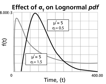
• The degree of skewness increases as [math]\displaystyle{ {{\sigma'}}\,\! }[/math] increases, for a given [math]\displaystyle{ \mu'\,\! }[/math]

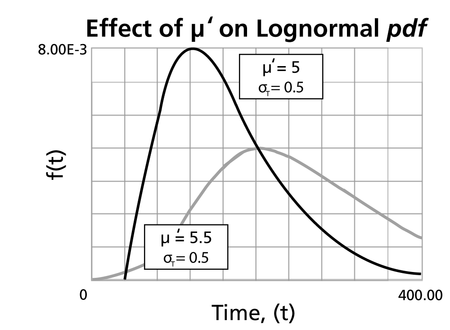
• For the same [math]\displaystyle{ {{\sigma'}}\,\! }[/math], the pdf 's skewness increases as [math]\displaystyle{ {\mu }'\,\! }[/math] increases.
• For [math]\displaystyle{ {{\sigma' }}\,\! }[/math] values significantly greater than 1, the pdf rises very sharply in the beginning, (i.e., for very small values of [math]\displaystyle{ T\,\! }[/math] near zero), and essentially follows the ordinate axis, peaks out early, and then decreases sharply like an exponential pdf or a Weibull pdf with [math]\displaystyle{ 0\lt \beta \lt 1\,\! }[/math].
• The parameter, [math]\displaystyle{ {\mu }'\,\! }[/math], in terms of the logarithm of the [math]\displaystyle{ {T}'s\,\! }[/math] is also the scale parameter, and not the location parameter as in the case of the normal pdf.
• The parameter [math]\displaystyle{ {{\sigma'}}\,\! }[/math], or the standard deviation of the [math]\displaystyle{ {T}'s\,\! }[/math] in terms of their logarithm or of their [math]\displaystyle{ {T}'\,\! }[/math], is also the shape parameter and not the scale parameter, as in the normal pdf, and assumes only positive values.

Lognormal Distribution Parameters in ReliaSoft's Software

In ReliaSoft's software, the parameters returned for the lognormal distribution are always logarithmic. That is: the parameter [math]\displaystyle{ {\mu }'\,\! }[/math] represents the mean of the natural logarithms of the times-to-failure, while [math]\displaystyle{ {{\sigma' }}\,\! }[/math] represents the standard deviation of these data point logarithms. Specifically, the returned [math]\displaystyle{ {{\sigma' }}\,\! }[/math] is the square root of the variance of the natural logarithms of the data points. Even though the application denotes these values as mean and standard deviation, the user is reminded that these are given as the parameters of the distribution, and are thus the mean and standard deviation of the natural logarithms of the data. The mean value of the times-to-failure, not used as a parameter, as well as the standard deviation can be obtained through the QCP or the Function Wizard.