|
|
| Line 114: |
Line 114: |
|
| |
|
|
| |
|
| [[Image:Non-Homogeneous Forecast Data.PNG|thumb|center|450px| ]] | | [[Image:Non-Homogeneous Forecast Data.PNG|thumb|center|550px| ]] |
|
| |
|
|
| |
|
| Line 126: |
Line 126: |
|
| |
|
|
| |
|
| [[Image:Non-Homogeneous Expected Failure.PNG|thumb|center|450px| ]] | | [[Image:Non-Homogeneous Expected Failure.PNG|thumb|center|550px| ]] |
Revision as of 07:46, 3 August 2012
New format available! This reference is now available in a new format that offers faster page load, improved display for calculations and images and more targeted search.
As of January 2024, this Reliawiki page will not continue to be updated. Please update all links and bookmarks to the latest references at Weibull examples and Weibull reference examples.
This example appears in the Life Data Analysis Reference book.
Warranty Analysis Non-Homogeneous Data Example
A company keeps track of its production and returns. The company uses the dates of failure format to record the data. For the product in question, three versions (A, B and C) have been produced and put in service. The in-service data is as follows (using the Month/Day/Year date format):
[math]\displaystyle{ \begin{matrix}
Quantity In-Service & Date of In-Service & ID \\
\text{400} & \text{1/1/2005} & \text{Model A} \\
\text{500} & \text{1/31/2005} & \text{Model A} \\
\text{500} & \text{5/1/2005} & \text{Model A} \\
\text{600} & \text{5/31/2005} & \text{Model A} \\
\text{550} & \text{6/30/2005} & \text{Model A} \\
\text{600} & \text{7/30/2005} & \text{Model A} \\
\text{800} & \text{9/28/2005} & \text{Model A} \\
\text{200} & \text{1/1/2005} & \text{Model B} \\
\text{350} & \text{3/2/2005} & \text{Model B} \\
\text{450} & \text{4/1/2005} & \text{Model B} \\
\text{300} & \text{6/30/2005} & \text{Model B} \\
\text{200} & \text{8/29/2005} & \text{Model B} \\
\text{350} & \text{10/28/2005} & \text{Model B} \\
\text{1100} & \text{2/1/2005} & \text{Model C} \\
\text{1200} & \text{3/27/2005} & \text{Model C} \\
\text{1200} & \text{4/25/2005} & \text{Model C} \\
\text{1300} & \text{6/1/2005} & \text{Model C} \\
\text{1400} & \text{8/26/2005} & \text{Model C} \\
\end{matrix} }[/math]
Furthermore, the following sales are forecast:
[math]\displaystyle{ \begin{matrix}
Number & Date & ID \\
\text{400} & \text{6/27/2006} & \text{Model A} \\
\text{500} & \text{8/26/2006} & \text{Model A} \\
\text{550} & \text{10/26/2006} & \text{Model A} \\
\text{1200} & \text{7/25/2006} & \text{Model C} \\
\text{1300} & \text{9/27/2006} & \text{Model C} \\
\text{1250} & \text{11/26/2006} & \text{Model C} \\
\end{matrix} }[/math]
The return data are as follows. Note that in order to identify which lot each unit comes from, and to be able to compute its time-in-service, each return (failure) includes a return date, the date of when it was put in service and the model ID.
[math]\displaystyle{ \begin{matrix}
Quantity Returned & Date of Return & Date In-Service & ID \\
\text{12} & \text{1/31/2005} & \text{1/1/2005} & \text{Model A} \\
\text{11} & \text{4/1/2005} & \text{1/31/2005} & \text{Model A} \\
\text{7} & \text{7/22/2005} & \text{5/1/2005} & \text{Model A} \\
\text{8} & \text{8/27/2005} & \text{5/31/2005} & \text{Model A} \\
\text{12} & \text{12/27/2005} & \text{5/31/2005} & \text{Model A} \\
\text{13} & \text{1/26/2006} & \text{6/30/2005} & \text{Model A} \\
\text{12} & \text{1/26/2006} & \text{7/30/2005} & \text{Model A} \\
\text{14} & \text{1/11/2006} & \text{9/28/2005} & \text{Model A} \\
\text{15} & \text{1/18/2006} & \text{9/28/2005} & \text{Model A} \\
\text{23} & \text{1/26/2005} & \text{1/1/2005} & \text{Model B} \\
\text{16} & \text{1/26/2005} & \text{1/1/2005} & \text{Model B} \\
\text{18} & \text{3/17/2005} & \text{1/1/2005} & \text{Model B} \\
\text{19} & \text{5/31/2005} & \text{3/2/2005} & \text{Model B} \\
\text{20} & \text{5/31/2005} & \text{3/2/2005} & \text{Model B} \\
\text{21} & \text{6/30/2005} & \text{3/2/2005} & \text{Model B} \\
\text{18} & \text{7/30/2005} & \text{4/1/2005} & \text{Model B} \\
\text{19} & \text{12/27/2005} & \text{6/30/2005} & \text{Model B} \\
\text{18} & \text{1/11/2006} & \text{8/29/2005} & \text{Model B} \\
\text{11} & \text{2/7/2006} & \text{10/28/2005} & \text{Model B} \\
\text{34} & \text{8/14/2005} & \text{3/27/2005} & \text{Model C} \\
\text{24} & \text{8/27/2005} & \text{4/25/2005} & \text{Model C} \\
\text{44} & \text{1/26/2006} & \text{6/1/2005} & \text{Model C} \\
\text{26} & \text{1/26/2006} & \text{8/26/2005} & \text{Model C} \\
\end{matrix} }[/math]
Assuming that the given information is current as of 5/1/2006, analyze the data using the lognormal distribution and MLE analysis method for all models (Model A, Model B, Model C), and provide a return forecast for the next ten months.
Solution
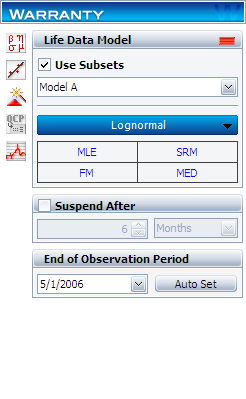
Create a warranty analysis folio and select the dates of failure format. Enter the data from the tables in the Sales, Returns and Future Sales sheets. On the control panel, select the Use Subsets check box, as shown next. This allows the software to separately analyze each subset of data. Use the drop-down list to switch between subset IDs and alter the analysis settings (use the lognormal distribution and MLE analysis method for all models).
In the End of Observation Period field, enter 5/1/2006, and then calculate the parameters. The results are:
[math]\displaystyle{ \begin{matrix}
Model A & Model B & Model C \\
\begin{matrix}
{{{\hat{\mu }}}^{\prime }}= & \text{11}\text{.28} \\
{{{\hat{\sigma }}}_{T}}= & \text{2}\text{.83} \\
\end{matrix} & \begin{matrix}
{{{\hat{\mu }}}^{\prime }}= & \text{8}\text{.11} \\
{{{\hat{\sigma }}}_{T}}= & \text{2}\text{.30} \\
\end{matrix} & \begin{matrix}
{{{\hat{\mu }}}^{\prime }}= & \text{9}\text{.79} \\
{{{\hat{\sigma }}}_{T}}= & \text{1}\text{.92} \\
\end{matrix} \\
\end{matrix} }[/math]
Note that in this example, the same distribution and analysis method were assumed for each of the product models. If desired, different distribution types, analysis methods, confidence bounds methods, etc., can be assumed for each IDs.
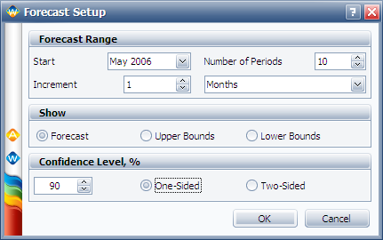
To obtain the expected failures for the next 10 months, click the Generate Forecast icon. In the Forecast Setup window, set the forecast to start on May 2, 2006 and set the number of forecast periods to 10. Set the increment (length of each period) to 1 Month, as shown next.
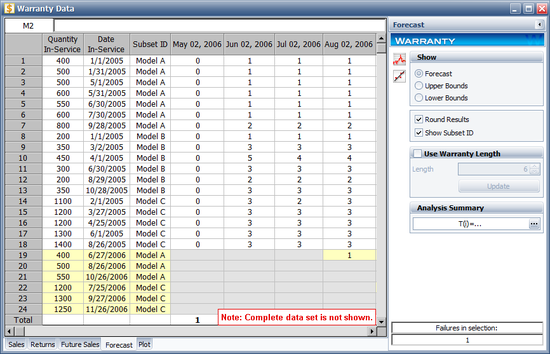
Click OK. A Forecast sheet will be created, with the predicted future returns. The following figure shows part of the Forecast sheet.
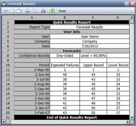
To view a summary of the analysis, click the Show Analysis Summary (...) button. The following figure shows the summary of the forecasted returns.
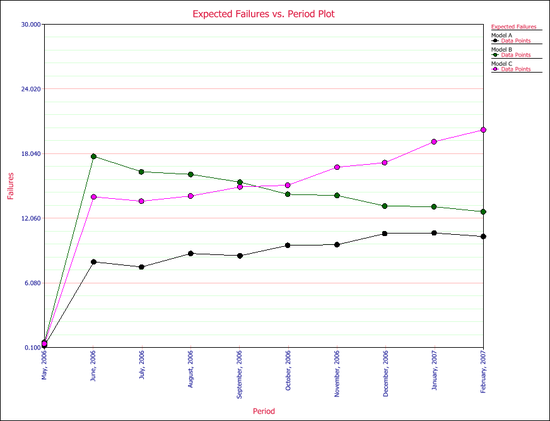
Click the Plot icon and choose the Expected Failures plot. The plot displays the predicted number of returns for each month, as shown next.

