Non-Homogeneous Data with Subset IDs Example

New format available! This reference is now available in a new format that offers faster page load, improved display for calculations and images and more targeted search.

As of January 2024, this Reliawiki page will not continue to be updated. Please update all links and bookmarks to the latest references at Weibull examples and Weibull reference examples.

---

This example appears in the Life Data Analysis Reference book.

Using Subset IDs with Statistical Process Control

A manufacturer wants to monitor and analyze the warranty returns for a particular product. They collected the following sales and return data.

[math]\displaystyle{ \begin{matrix} Period & Quantity In-Service \\ \text{Sep 04} & \text{1150} \\ \text{Oct 04} & \text{1100} \\ \text{Nov 04} & \text{1200} \\ \text{Dec 04} & \text{1155} \\ \text{Jan 05} & \text{1255} \\ \text{Feb 05} & \text{1150} \\ \text{Mar 05} & \text{1105} \\ \text{Apr 05} & \text{1110} \\ \end{matrix} }[/math]

[math]\displaystyle{ \begin{matrix} {} & Oct 04 & Nov 04 & Dec 04 & Jan 05 & Feb 05 & Mar 05 & Apr 05 & May 05 \\ Sep 05 & \text{2} & \text{4} & \text{5} & \text{7} & \text{12} & \text{13} & \text{16} & \text{17} \\ Oct 05 & \text{-} & \text{3} & \text{4} & \text{5} & \text{3} & \text{8} & \text{11} & \text{14} \\ Nov 05 & \text{-} & \text{-} & \text{2} & \text{3} & \text{5} & \text{7} & \text{23} & \text{13} \\ Dec 05 & \text{-} & \text{-} & \text{-} & \text{2} & \text{3} & \text{4} & \text{6} & \text{7} \\ Jan 06 & \text{-} & \text{-} & \text{-} & \text{-} & \text{2} & \text{3} & \text{3} & \text{4} \\ Feb 06 & \text{-} & \text{-} & \text{-} & \text{-} & \text{-} & \text{2} & \text{3} & \text{3} \\ Mar 06 & \text{-} & \text{-} & \text{-} & \text{-} & \text{-} & \text{-} & \text{2} & \text{12} \\ Apr 06 & \text{-} & \text{-} & \text{-} & \text{-} & \text{-} & \text{-} & \text{-} & \text{2} \\ \end{matrix} }[/math]

Solution

Analyze the data using the two-parameter Weibull distribution and the MLE analysis method. The parameters are estimated to be:

[math]\displaystyle{ \begin{align} & & \beta = & 2.318144 \\ & & \eta = & 25.071878 \end{align} }[/math]

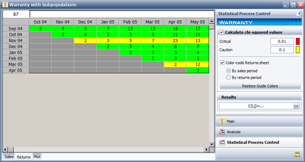
To analyze the warranty returns, select the check box in the Statistical Process Control page of the control panel and set the alpha values to 0.01 for the Critical Value and 0.1 for the Caution Value. Select to color code the results By sales period. The following figure shows the analysis settings and results of the analysis.

As you can see, the November 04 and March 05 sales periods are colored in yellow indicating that they are outlier sales periods, while the rest are green. One suspected reason for the variation may be the material used in production during these periods. Further analysis confirmed that for these periods, the material was acquired from a different supplier. This implies that the units are not homogenous, and that there are different sub-populations present in the field population.

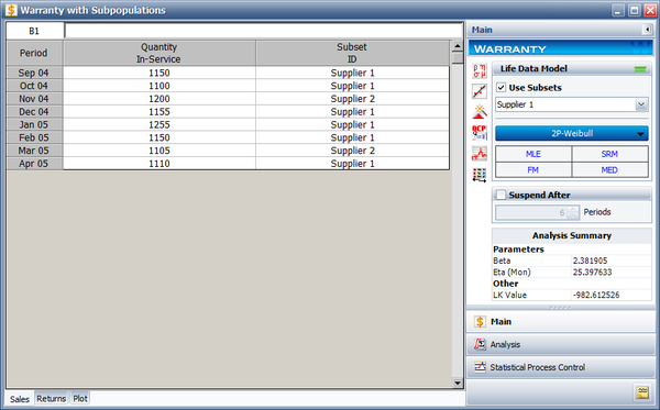
Categorized each shipment (using the Subset ID column) based on their material supplier, as shown next. On the control panel, select the Use Subsets check box. Perform the analysis again using the two-parameter Weibull distribution and the MLE analysis method for both sub-populations.

The new models that describe the data are:

[math]\displaystyle{ \begin{matrix} Supplier 1 & Supplier 2 \\ \begin{matrix} \beta =2.381905 \\ \eta =25.397633 \\ \end{matrix} & \begin{matrix} \beta =2.320696 \\ \eta =21.282926 \\ \end{matrix} \\ \end{matrix} }[/math]

This analysis uncovered different sub-populations in the data set. Note that if the analysis were performed on the failure and suspension times in a regular standard folio using the mixed Weibull distribution, one would not be able to detect which units fall into which sub-population.