2P Exponential Example: Difference between revisions
Lisa Hacker (talk | contribs) No edit summary |
Kate Racaza (talk | contribs) (Started review. Will need theory input) |
||
| Line 1: | Line 1: | ||
{{Banner Weibull Examples}} | <noinclude>{{Banner Weibull Examples}}[[Category:NTI]]</noinclude> | ||
'''2 Parameter Exponential Distribution RRY''' | '''2 Parameter Exponential Distribution RRY''' | ||
Fourteen units were | Fourteen units were reliability tested and the following life test data were obtained: | ||
| Line 42: | Line 41: | ||
|14 ||100 | |14 ||100 | ||
|} | |} | ||
Assuming that the data follow a two-parameter exponential distribution, estimate the parameters and determine the correlation coefficient, <math>\rho </math>, using rank regression on Y. | Assuming that the data follow a two-parameter exponential distribution, estimate the parameters and determine the correlation coefficient, <math>\rho </math>, using rank regression on Y. | ||
'''Solution''' | '''Solution''' | ||
Construct | Construct a table, as shown next. | ||
<center><math>\overset{{}}{\mathop{\text{Table}\text{- Least Squares Analysis}}}\,</math></center> | <center><math>\overset{{}}{\mathop{\text{Table}\text{- Least Squares Analysis}}}\,</math></center> | ||
| Line 71: | Line 72: | ||
The median rank values ( <math>F({{t}_{i}})</math> ) can be found in rank tables or they can be estimated using the '''Quick Statistical Reference''' in Weibull++. | The median rank values ( <math>F({{t}_{i}})</math> ) can be found in rank tables or they can be estimated using the '''Quick Statistical Reference (QSR)''' tool in Weibull++. | ||
Given the values in the table above, calculate <math>\hat{a}</math> and <math>\hat{b}</math>: | Given the values in the table above, calculate <math>\hat{a}</math> and <math>\hat{b}</math>: | ||
| Line 112: | Line 113: | ||
The correlation coefficient can be estimated using equation for calculating the correlation coefficient: | The correlation coefficient can be estimated using the equation for calculating the correlation coefficient: | ||
::<math>\hat{\rho }=-0.9679</math> | ::<math>\hat{\rho }=-0.9679</math> | ||
This example can be repeated using Weibull++ | This example can be repeated using Weibull++ by choosing the two-parameter exponential distribution and the rank regression on Y (RRY) parameter estimation method. The estimated parameters and the correlation coefficient are <math>\hat{\lambda }=0.0271\text{ fr/hr },\hat{\gamma }=10.1348\text{ hr },\hat{\rho }=-0.9679</math>, as shown next. | ||
[[Image:Exponential Example 2 Data Folio.png|thumb|center|400px|]] | |||
Please note that the user must deselect the '''Reset if Loc. Param > T1 on Exp RR''' option on the user setup page. | |||
The probability plot can be obtained simply by clicking the '''Plot''' icon. | The probability plot can be obtained simply by clicking the '''Plot''' icon. | ||
[[Image:Exponential Example 2 Plot.png|thumb|center|400px|]] | [[Image:Exponential Example 2 Plot.png|thumb|center|400px|]] | ||
Revision as of 10:57, 20 July 2012
New format available! This reference is now available in a new format that offers faster page load, improved display for calculations and images and more targeted search.
As of January 2024, this Reliawiki page will not continue to be updated. Please update all links and bookmarks to the latest references at Weibull examples and Weibull reference examples.
2 Parameter Exponential Distribution RRY
Fourteen units were reliability tested and the following life test data were obtained:
| Table - Life Test Data | |
| Data point index | Time-to-failure |
|---|---|
| 1 | 5 |
| 2 | 10 |
| 3 | 15 |
| 4 | 20 |
| 5 | 25 |
| 6 | 30 |
| 7 | 35 |
| 8 | 40 |
| 9 | 50 |
| 10 | 60 |
| 11 | 70 |
| 12 | 80 |
| 13 | 90 |
| 14 | 100 |
Assuming that the data follow a two-parameter exponential distribution, estimate the parameters and determine the correlation coefficient, [math]\displaystyle{ \rho }[/math], using rank regression on Y.
Solution
Construct a table, as shown next.
The median rank values ( [math]\displaystyle{ F({{t}_{i}}) }[/math] ) can be found in rank tables or they can be estimated using the Quick Statistical Reference (QSR) tool in Weibull++.
Given the values in the table above, calculate [math]\displaystyle{ \hat{a} }[/math] and [math]\displaystyle{ \hat{b} }[/math]:
- [math]\displaystyle{ \begin{align} \hat{b}= & \frac{\underset{i=1}{\overset{14}{\mathop{\sum }}}\,{{t}_{i}}{{y}_{i}}-(\underset{i=1}{\overset{14}{\mathop{\sum }}}\,{{t}_{i}})(\underset{i=1}{\overset{14}{\mathop{\sum }}}\,{{y}_{i}})/14}{\underset{i=1}{\overset{14}{\mathop{\sum }}}\,t_{i}^{2}-{{(\underset{i=1}{\overset{14}{\mathop{\sum }}}\,{{t}_{i}})}^{2}}/14} \\ \\ \hat{b}= & \frac{-927.4899-(630)(-13.2315)/14}{40,600-{{(630)}^{2}}/14} \end{align} }[/math]
or:
- [math]\displaystyle{ \hat{b}=-0.02711 }[/math]
and:
- [math]\displaystyle{ \hat{a}=\overline{y}-\hat{b}\overline{t}=\frac{\underset{i=1}{\overset{N}{\mathop{\sum }}}\,{{y}_{i}}}{N}-\hat{b}\frac{\underset{i=1}{\overset{N}{\mathop{\sum }}}\,{{t}_{i}}}{N} }[/math]
or:
- [math]\displaystyle{ \hat{a}=\frac{-13.2315}{14}-(-0.02711)\frac{630}{14}=0.2748 }[/math]
Therefore:
- [math]\displaystyle{ \hat{\lambda }=-\hat{b}=-(-0.02711)=0.02711\text{ failures/hour} }[/math]
and:
- [math]\displaystyle{ \hat{\gamma }=\frac{\hat{a}}{\hat{\lambda }}=\frac{0.2748}{0.02711} }[/math]
or:
- [math]\displaystyle{ \hat{\gamma }=10.1365\text{ hours} }[/math]
Then:
- [math]\displaystyle{ f(t)=(0.02711)\cdot {{e}^{-0.02711(T-10.136)}} }[/math]
The correlation coefficient can be estimated using the equation for calculating the correlation coefficient:
- [math]\displaystyle{ \hat{\rho }=-0.9679 }[/math]
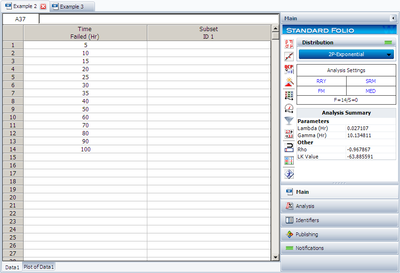
This example can be repeated using Weibull++ by choosing the two-parameter exponential distribution and the rank regression on Y (RRY) parameter estimation method. The estimated parameters and the correlation coefficient are [math]\displaystyle{ \hat{\lambda }=0.0271\text{ fr/hr },\hat{\gamma }=10.1348\text{ hr },\hat{\rho }=-0.9679 }[/math], as shown next.
Please note that the user must deselect the Reset if Loc. Param > T1 on Exp RR option on the user setup page.
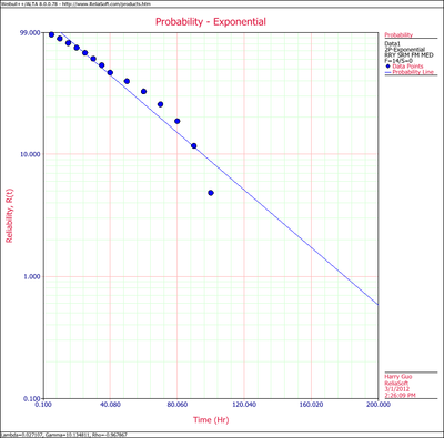
The probability plot can be obtained simply by clicking the Plot icon.


