Tensile Components Example: Difference between revisions
(Created page with '===Tensile Components Example=== A tensile component of a landing gear was put through an accelerated reliability test to determine whether the life goal would be achieved unde…') |
Chris Kahn (talk | contribs) |
||
| Line 60: | Line 60: | ||
<br> | <br> | ||
[[Image:new_3.gif|thumb|center| | [[Image:new_3.gif|thumb|center|500px|Probability plots at different shock loads.]] | ||
<br> | <br> | ||
| Line 66: | Line 66: | ||
<br> | <br> | ||
[[Image:new_4.gif|thumb|center| | [[Image:new_4.gif|thumb|center|500px|The probability plot at a use stress level of 50 kips.]] | ||
<br> | <br> | ||
| Line 73: | Line 73: | ||
<br> | <br> | ||
[[Image:ipl_example_specify_life.gif|thumb|center| | [[Image:ipl_example_specify_life.gif|thumb|center|500px|]] | ||
<br> | <br> | ||
| Line 79: | Line 79: | ||
<br> | <br> | ||
[[Image:new_5.gif|thumb|center| | [[Image:new_5.gif|thumb|center|500px|Median Life line (right) and 10% unreliability line (left) vs. stress.]] | ||
<br> | <br> | ||
| Line 85: | Line 85: | ||
<br> | <br> | ||
[[Image:ipl_example2_qcp.gif|thumb|center| | [[Image:ipl_example2_qcp.gif|thumb|center|500px|]] | ||
<br> | <br> | ||
The design criterion of 10,000 landings is met. | The design criterion of 10,000 landings is met. | ||
Revision as of 13:19, 25 June 2012
Tensile Components Example
A tensile component of a landing gear was put through an accelerated reliability test to determine whether the life goal would be achieved under the designed-in load. Fifteen units, N=15, were tested at three different shock loads. The component was designed for a peak shock load of 50 kips with an estimated return of 10% of the population by 10,000 landings. Using the inverse power law lognormal model, determine whether the design life was met.
| Failure, in Cycles | Shock Load, kips |
|---|---|
| 1855 | 73 |
| 2158 | 73 |
| 2425 | 73 |
| 2736 | 73 |
| 3206 | 73 |
| 614 | 95 |
| 770 | 95 |
| 781 | 95 |
| 890 | 95 |
| 1055 | 95 |
| 152 | 128 |
| 162 | 128 |
| 173 | 128 |
| 209 | 128 |
| 216 | 128 |
Solution
The data were entered into ALTA, and the following estimates were obtained for the parameters of the IPL-lognormal model:
- [math]\displaystyle{ \begin{align} Std=\ & 0.179080 \\ K=\ & 8.953055E-13 \\ n=\ & 4.638882 \end{align} }[/math]
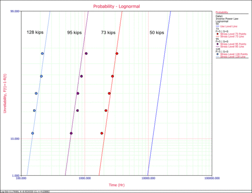
The probability plot at each test stress level (73 kips, 95 kips and 123 kips) was then obtained, as shown next.
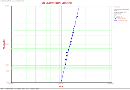
In this plot, it can be seen that there is a good agreement between the data and the fitted model. The probability plot at a use stress level of 50 kips is shown next.
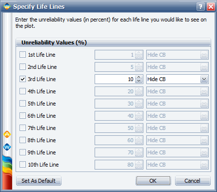
Using the Use Level Probability plot, the cycles-to failure for a 10% probability of failure can be estimated. From the plot, this time is estimated to be [math]\displaystyle{ T(Q=0.10=10%)\approxeq 12,000 }[/math] landings. Another way to obtain life information is by using a Life vs. Stress plot. Once a Life vs. Stress plot is selected, the 10% unreliability (probability of failure) line must be plotted. To do this, click Life Lines... in the plot panel and and select the 10% Unreliability box (or enter 10 in one of the boxes and select the box) in the Specify Life Lines window, as shown next.
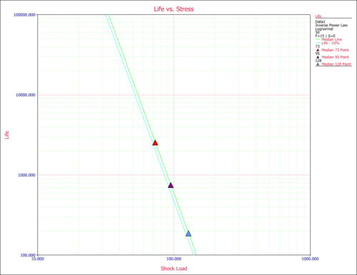
In the following plot, the 10% unreliability line is plotted (the first line from the left). For a stress of 50 psi (X-axis) and for the 10% unreliability line, the cycles-to-failure can be obtained by reading the value on the Y-axis. Again, [math]\displaystyle{ T(0.1)\approxeq 12,000 }[/math] landings.
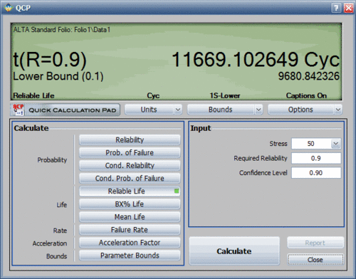
However, a more accurate way to obtain such information is by using the Quick Calculation Pad (QCP) in ALTA. Using the QCP, the life for a 10% probability of failure at 50 kips is estimated to be 11,669.1 cycles (or landings), as shown next.
The design criterion of 10,000 landings is met.
