Eyring Relationship: Difference between revisions
Lisa Hacker (talk | contribs) No edit summary |
Lisa Hacker (talk | contribs) No edit summary |
||
| Line 64: | Line 64: | ||
{{eyring confidence bounds}} | {{eyring confidence bounds}} | ||
Revision as of 17:58, 6 June 2012
Introduction
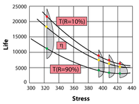
The Eyring relationship was formulated from quantum mechanics principles [9] and is most often used when thermal stress (temperature) is the acceleration variable. However, the Eyring relationship is also often used for stress variables other than temperature, such as humidity. The relationship is given by:
- [math]\displaystyle{ L(V)=\frac{1}{V}{{e}^{-\left( A-\tfrac{B}{V} \right)}} }[/math]
where:
• [math]\displaystyle{ L }[/math] represents a quantifiable life measure, such as mean life, characteristic life, median life, [math]\displaystyle{ B(x) }[/math] life, etc.
• [math]\displaystyle{ V }[/math] represents the stress level (temperature values are in absolute units: kelvin or degrees Rankine).
• [math]\displaystyle{ A }[/math] is one of the model parameters to be determined.
• [math]\displaystyle{ B }[/math] is another model parameter to be determined.
The Eyring relationship is similar to the Arrhenius relationship. This similarity is more apparent if it is rewritten in the following way:
- [math]\displaystyle{ \begin{align} L(V)=\ & \frac{1}{V}{{e}^{-\left( A-\tfrac{B}{V} \right)}} =\ & \frac{{{e}^{-A}}}{V}{{e}^{\tfrac{B}{V}}} \end{align} }[/math]
or:
- [math]\displaystyle{ L(V)=\frac{1}{V}Const.\cdot {{e}^{\tfrac{B}{V}}} }[/math]
The Arrhenius relationship is given by:
- [math]\displaystyle{ L(V)=C\cdot {{e}^{\tfrac{B}{V}}} }[/math]
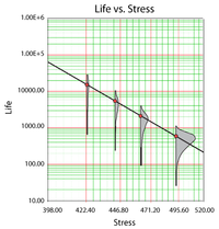
Comparing the above equation to the Arrhenius relationship, it can be seen that the only difference between the two relationships is the [math]\displaystyle{ \tfrac{1}{V} }[/math] term above. In general, both relationships yield very similar results. Like the Arrhenius, the Eyring relationship is plotted on a log-reciprocal paper.
Template loop detected: Template:Alta e.a-e acceleration factor
Template loop detected: Template:Alta a-e.e-e
Template loop detected: Template:Alta eyring-weibull
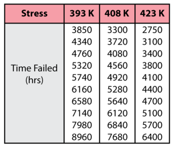
Consider the following times-to-failure data at three different stress levels.
The data set was entered into the ALTA standard folio and analyzed using the Eyring-Weibull model, yielding:
- [math]\displaystyle{ \widehat{\beta }=4.29186497\,\! }[/math]
- [math]\displaystyle{ \widehat{A}=-11.08784624\,\! }[/math]
- [math]\displaystyle{ \widehat{B}=1454.08635742\,\! }[/math]
Once the parameters of the model are defined, other life measures can be directly obtained using the appropriate equations. For example, the MTTF can be obtained for the use stress level of 323 K by using:
- [math]\displaystyle{ \overline{T}=\frac{1}{V}{{e}^{-\left( A-\tfrac{B}{V} \right)}}\cdot \Gamma \left( \frac{1}{\beta }+1 \right)\,\! }[/math]
or:
- [math]\displaystyle{ \begin{align} & \overline{T}= & \frac{1}{323}{{e}^{-\left( -11.08784624-\tfrac{1454.08635742}{323} \right)}}\cdot \Gamma \left( \frac{1}{4.29186497}+1 \right) =16,610\text{ }hr \end{align}\,\! }[/math]
Template loop detected: Template:Erying-log
Template loop detected: Template:Generalized eyring
Template loop detected: Template:Eyring confidence bounds
Consider the following times-to-failure data at three different stress levels.
The data set was entered into the ALTA standard folio and analyzed using the Eyring-Weibull model, yielding:
- [math]\displaystyle{ \widehat{\beta }=4.29186497\,\! }[/math]
- [math]\displaystyle{ \widehat{A}=-11.08784624\,\! }[/math]
- [math]\displaystyle{ \widehat{B}=1454.08635742\,\! }[/math]
Once the parameters of the model are defined, other life measures can be directly obtained using the appropriate equations. For example, the MTTF can be obtained for the use stress level of 323 K by using:
- [math]\displaystyle{ \overline{T}=\frac{1}{V}{{e}^{-\left( A-\tfrac{B}{V} \right)}}\cdot \Gamma \left( \frac{1}{\beta }+1 \right)\,\! }[/math]
or:
- [math]\displaystyle{ \begin{align} & \overline{T}= & \frac{1}{323}{{e}^{-\left( -11.08784624-\tfrac{1454.08635742}{323} \right)}}\cdot \Gamma \left( \frac{1}{4.29186497}+1 \right) =16,610\text{ }hr \end{align}\,\! }[/math]
Introduction
The Eyring relationship was formulated from quantum mechanics principles [9] and is most often used when thermal stress (temperature) is the acceleration variable. However, the Eyring relationship is also often used for stress variables other than temperature, such as humidity. The relationship is given by:
- [math]\displaystyle{ L(V)=\frac{1}{V}{{e}^{-\left( A-\tfrac{B}{V} \right)}} }[/math]
where:
• [math]\displaystyle{ L }[/math] represents a quantifiable life measure, such as mean life, characteristic life, median life, [math]\displaystyle{ B(x) }[/math] life, etc.
• [math]\displaystyle{ V }[/math] represents the stress level (temperature values are in absolute units: kelvin or degrees Rankine).
• [math]\displaystyle{ A }[/math] is one of the model parameters to be determined.
• [math]\displaystyle{ B }[/math] is another model parameter to be determined.
The Eyring relationship is similar to the Arrhenius relationship. This similarity is more apparent if it is rewritten in the following way:
- [math]\displaystyle{ \begin{align} L(V)=\ & \frac{1}{V}{{e}^{-\left( A-\tfrac{B}{V} \right)}} =\ & \frac{{{e}^{-A}}}{V}{{e}^{\tfrac{B}{V}}} \end{align} }[/math]
or:
- [math]\displaystyle{ L(V)=\frac{1}{V}Const.\cdot {{e}^{\tfrac{B}{V}}} }[/math]
The Arrhenius relationship is given by:
- [math]\displaystyle{ L(V)=C\cdot {{e}^{\tfrac{B}{V}}} }[/math]
Comparing the above equation to the Arrhenius relationship, it can be seen that the only difference between the two relationships is the [math]\displaystyle{ \tfrac{1}{V} }[/math] term above. In general, both relationships yield very similar results. Like the Arrhenius, the Eyring relationship is plotted on a log-reciprocal paper.
Template loop detected: Template:Alta e.a-e acceleration factor
Template loop detected: Template:Alta a-e.e-e
Template loop detected: Template:Alta eyring-weibull
Consider the following times-to-failure data at three different stress levels.
The data set was entered into the ALTA standard folio and analyzed using the Eyring-Weibull model, yielding:
- [math]\displaystyle{ \widehat{\beta }=4.29186497\,\! }[/math]
- [math]\displaystyle{ \widehat{A}=-11.08784624\,\! }[/math]
- [math]\displaystyle{ \widehat{B}=1454.08635742\,\! }[/math]
Once the parameters of the model are defined, other life measures can be directly obtained using the appropriate equations. For example, the MTTF can be obtained for the use stress level of 323 K by using:
- [math]\displaystyle{ \overline{T}=\frac{1}{V}{{e}^{-\left( A-\tfrac{B}{V} \right)}}\cdot \Gamma \left( \frac{1}{\beta }+1 \right)\,\! }[/math]
or:
- [math]\displaystyle{ \begin{align} & \overline{T}= & \frac{1}{323}{{e}^{-\left( -11.08784624-\tfrac{1454.08635742}{323} \right)}}\cdot \Gamma \left( \frac{1}{4.29186497}+1 \right) =16,610\text{ }hr \end{align}\,\! }[/math]
Template loop detected: Template:Erying-log
Template loop detected: Template:Generalized eyring
Template loop detected: Template:Eyring confidence bounds


