Template:Three-parameter weibull regression: Difference between revisions
No edit summary |
|||
| Line 3: | Line 3: | ||
When the MR versus <span class="texhtml">''t''<sub>''j''</sub></span> points plotted on the Weibull probability paper do not fall on a satisfactory straight line and the points fall on a curve,(Note that other shapes, particularly shapes, might suggest the existence of more than one population. In these cases, the multiple population, mixed Weibull distribution, may be more appropriate. Chapter [[The Mixed Weibull Distribution]] presents the mixed Weibull distribution.) then a location parameter, <span class="texhtml">γ</span>, might exist which may straighten out these points. The goal in this case is to fit a curve, instead of a line, through the data points using nonlinear regression. The Gauss-Newton method can be used to solve for the parameters, <span class="texhtml">β</span>, <span class="texhtml">η</span> and <span class="texhtml">γ</span>, by performing a Taylor series expansion on <span class="texhtml">''F''(''t''<sub>''i''</sub>;β,η,γ)</span>. Then the nonlinear model is approximated with linear terms and ordinary least squares are employed to estimate the parameters. This procedure is iterated until a satisfactory solution is reached. Weibull++ calculates the value of <span class="texhtml">γ</span> by utilizing an optimized Nelder-Mead algorithm, and adjusts the points by this value of <span class="texhtml">γ</span> such that they fall on a straight line, and then plots both the adjusted and the original unadjusted points. To draw a curve through the original unadjusted points, if so desired, select Weibull 3P Line Unadjusted for Gamma from the ''Show Plot Line'' submenu under the ''Plot Options'' menu. The returned estimations of the parameters are the same when selecting RRX or RRY. To display the unadjusted data points and line along with the adjusted data points and line, select ''Show/Hide Items'' under the ''Plot Options ''menu and include the unadjusted data points and line as follows: | When the MR versus <span class="texhtml">''t''<sub>''j''</sub></span> points plotted on the Weibull probability paper do not fall on a satisfactory straight line and the points fall on a curve,(Note that other shapes, particularly shapes, might suggest the existence of more than one population. In these cases, the multiple population, mixed Weibull distribution, may be more appropriate. Chapter [[The Mixed Weibull Distribution]] presents the mixed Weibull distribution.) then a location parameter, <span class="texhtml">γ</span>, might exist which may straighten out these points. The goal in this case is to fit a curve, instead of a line, through the data points using nonlinear regression. The Gauss-Newton method can be used to solve for the parameters, <span class="texhtml">β</span>, <span class="texhtml">η</span> and <span class="texhtml">γ</span>, by performing a Taylor series expansion on <span class="texhtml">''F''(''t''<sub>''i''</sub>;β,η,γ)</span>. Then the nonlinear model is approximated with linear terms and ordinary least squares are employed to estimate the parameters. This procedure is iterated until a satisfactory solution is reached. Weibull++ calculates the value of <span class="texhtml">γ</span> by utilizing an optimized Nelder-Mead algorithm, and adjusts the points by this value of <span class="texhtml">γ</span> such that they fall on a straight line, and then plots both the adjusted and the original unadjusted points. To draw a curve through the original unadjusted points, if so desired, select Weibull 3P Line Unadjusted for Gamma from the ''Show Plot Line'' submenu under the ''Plot Options'' menu. The returned estimations of the parameters are the same when selecting RRX or RRY. To display the unadjusted data points and line along with the adjusted data points and line, select ''Show/Hide Items'' under the ''Plot Options ''menu and include the unadjusted data points and line as follows: | ||
[[Image:showhideplotitems.png | [[Image:showhideplotitems.png|center|200px]] | ||
[[Image:Weibull Distribution Example 4 Show Hide Items.png|thumb|center|300px]] | [[Image:Weibull Distribution Example 4 Show Hide Items.png|thumb|center|300px]] | ||
Revision as of 18:15, 25 April 2012
Three-Parameter Weibull Regression
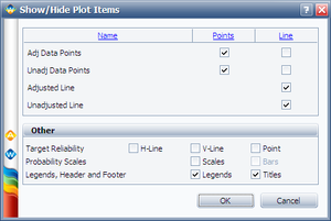
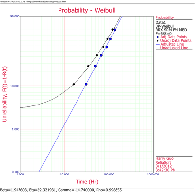
When the MR versus tj points plotted on the Weibull probability paper do not fall on a satisfactory straight line and the points fall on a curve,(Note that other shapes, particularly shapes, might suggest the existence of more than one population. In these cases, the multiple population, mixed Weibull distribution, may be more appropriate. Chapter The Mixed Weibull Distribution presents the mixed Weibull distribution.) then a location parameter, γ, might exist which may straighten out these points. The goal in this case is to fit a curve, instead of a line, through the data points using nonlinear regression. The Gauss-Newton method can be used to solve for the parameters, β, η and γ, by performing a Taylor series expansion on F(ti;β,η,γ). Then the nonlinear model is approximated with linear terms and ordinary least squares are employed to estimate the parameters. This procedure is iterated until a satisfactory solution is reached. Weibull++ calculates the value of γ by utilizing an optimized Nelder-Mead algorithm, and adjusts the points by this value of γ such that they fall on a straight line, and then plots both the adjusted and the original unadjusted points. To draw a curve through the original unadjusted points, if so desired, select Weibull 3P Line Unadjusted for Gamma from the Show Plot Line submenu under the Plot Options menu. The returned estimations of the parameters are the same when selecting RRX or RRY. To display the unadjusted data points and line along with the adjusted data points and line, select Show/Hide Items under the Plot Options menu and include the unadjusted data points and line as follows:


The results and the associated graph for the previous example using the three-parameter Weibull case are shown next:
