Complex Failure Modes Example: Difference between revisions
No edit summary |
No edit summary |
||
| Line 20: | Line 20: | ||
<math></math> | <math></math> | ||
[[Image: | [[Image:WB.18 RBD.png|center|400px| ]] | ||
One folio with multiple data sheets was created in Weibull++ for each of the data sets and each file was analyzed using the two-parameter Weibull distribution, MLE as the analysis method and Fisher Matrix as the confidence bounds method. A diagram is created by choosing '''Diagram''' from the Insert menu. The failure modes can be inserted into the diagram by selecting them from the '''Adding Block''' window. | One folio with multiple data sheets was created in Weibull++ for each of the data sets and each file was analyzed using the two-parameter Weibull distribution, MLE as the analysis method and Fisher Matrix as the confidence bounds method. A diagram is created by choosing '''Diagram''' from the Insert menu. The failure modes can be inserted into the diagram by selecting them from the '''Adding Block''' window. | ||
Revision as of 16:31, 15 March 2012
Competing Failures with Complex Configuration Example
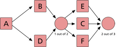
Assume that a product has five failure modes: A, B, C, D and F. Furthermore, assume that failure of the product will occur if mode A occurs, modes B and C occur simultaneously or if either modes C and D, C and F or D and F occur simultaneously. Times-to-failure for each mode is given in the next table.
The RBD that describes this configuration is shown next.
[math]\displaystyle{ }[/math]
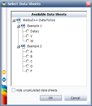
One folio with multiple data sheets was created in Weibull++ for each of the data sets and each file was analyzed using the two-parameter Weibull distribution, MLE as the analysis method and Fisher Matrix as the confidence bounds method. A diagram is created by choosing Diagram from the Insert menu. The failure modes can be inserted into the diagram by selecting them from the Adding Block window.
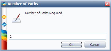
The nodes are inserted by clicking choosing Add Node from the Diagram menu. The number of required paths can be specified by double clicking the node and entering the appropriate number (1 in the first node and 2 in the second node).
[math]\displaystyle{ }[/math]
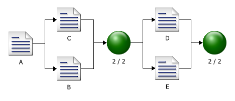
The diagam is:
[math]\displaystyle{ }[/math]
Using the Quick Calculation Pad (QCP), the estimated R( [math]\displaystyle{ 100 }[/math] hours [math]\displaystyle{ ) }[/math] and the 90% two-sided confidence bounds are:
- [math]\displaystyle{ \begin{matrix} {{{\hat{R}}}_{U}}(100)=0.991 \\ \hat{R}(100)=0.9905 \\ {{{\hat{R}}}_{L}}(100)=0.9080 \\ \end{matrix} }[/math]


