Template:Weibull++ SimuMatic Example: Difference between revisions
Created page with ''''Example of Using Weibull++ SimuMatic ''' SimuMatic is a simulation tool in Weibull++. It can be used to design life tests, reliability demonstration tests, and study the effe…' |
No edit summary |
||
| Line 29: | Line 29: | ||
[[image: SimuMatic Setup Distribution updated.png|thumb|center|400px]] | [[image: SimuMatic Setup Distribution updated.png|thumb|center|400px]] | ||
Step 3: Set up the rest inputs for SimuMatic using the following settings. | '''Step 3:''' Set up the rest inputs for SimuMatic using the following settings. | ||
[[image: SimuMatic Setup censoring.png|thumb|center|400px]] | [[image: SimuMatic Setup censoring.png|thumb|center|400px]] | ||
Revision as of 18:05, 7 March 2012
Example of Using Weibull++ SimuMatic
SimuMatic is a simulation tool in Weibull++. It can be used to design life tests, reliability demonstration tests, and study the effect of sample size.
Assume an engineer wants to design a test to estimate the B10 life a product. He knows large test sample size will provide more confidence on the analysis results from the test outcome. In other words, large sample size will narrow the confidence interval of the estimated B10 life. If he wants the ratio of the estimated one-sided upper and lower confidence bounds at a confidence level of 90% to be less than 1.5, how many samples he need to test?
The needed sample size can be found using SimuMatic in Weibull++.
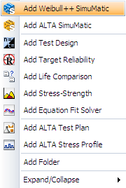
Step 1: To use Simumatic, select Add Weibull++ SimuMatic from the Tools from the Project Explore.
Step 2: In order to simulate random data, a distribution must be assumed. This is set in the following window.
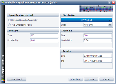
The engineer knows that by time 200, probably 1 out of 100 test units will fail; by time 300, probably 4 out of 100 test units will fail. Based on this information, the Quick Parameter Estimator can generate the parameters for a specified distribution.
Click on the Quick Parameter Estimator, enter the above information, and calculated the distribution parameters. The result is given at:

Click on Update, the solved parameters become the inputs for the SimuMatic:

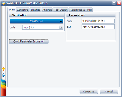
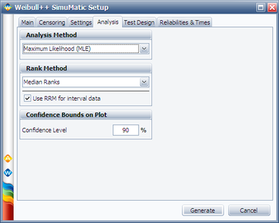
Step 3: Set up the rest inputs for SimuMatic using the following settings.
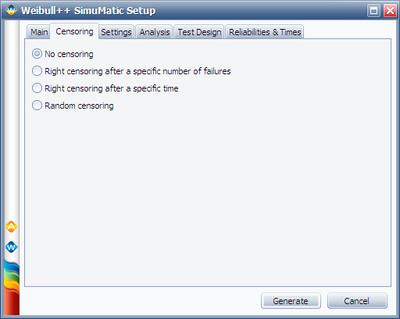
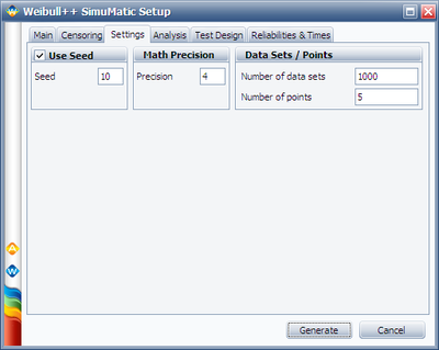
Initially, we used 5 as the initial guess for the sample size. This value should be adjusted based on calculated confidence bound ratio. If the ratio is bigger than the required value of 1.5, we should increase it; if the ratio is smaller than the required value of 1.5, we should decrease it. By trial and error, we can find the most appropriate value for sample size.
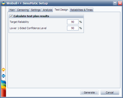
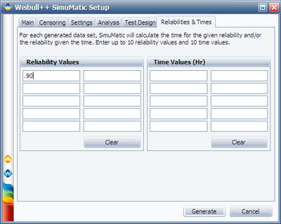
In the above figure, we set Reliability value = 0.9 because we need to estimate the B10 life of the product.
Step 4: Click on Generate to generate the data and review the results. Two sheets were generated for the results. In the Simulation Sheet, the estimated results for each generated data set were given. In the Sorted sheet, results are sorted. It is shown below.
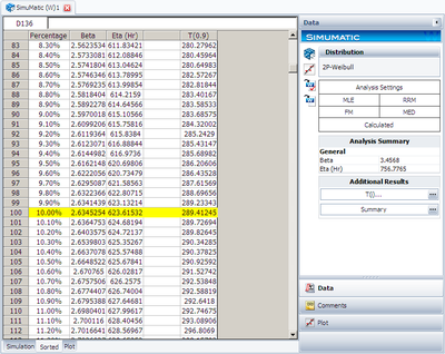
In above figure, the 10% percentile of the calculated B10 life (Reliability = 0.9). From the above result, we can see the lower bound of the B10 life is 289.41. Similarly, we can find the upper bound to be:
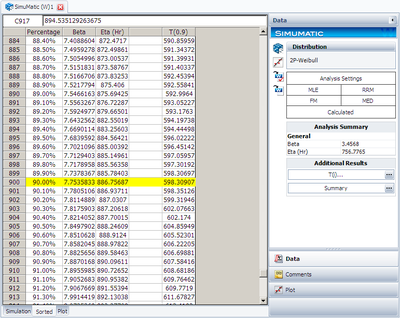
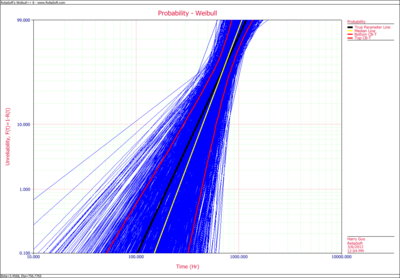
The ratio of these two bounds is 598.31/289.41 = 2.07, which is bigger than the required value of 1.5. Therefore, we need to increase the sample size. The simulation result and the confidence bounds are also can be viewed at the following plot.
Step 5: Increase sample size and calculate the confidence bound ratio until find an appropriate sample size. When the sample size is 18, the calculated bound ratio is 1.502. The results are:
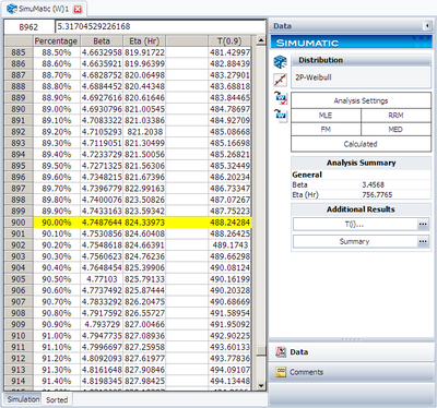
The plot is:
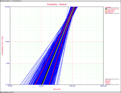
Compare this figure with the plot for sample size of 5, it can be seen that the confidence interval is much narrow.
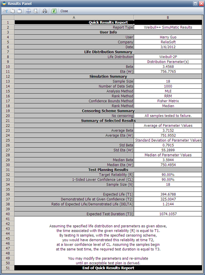
Therefore, using SimuMatic we found the suitable sample size of 18. There are many other results in SimuMatic. Click on the 'Summary… button, you can view the summary.
