Time-Dependent System Reliability (Analytical)

In the previous chapter, different system configuration types were examined, as well as different methods for obtaining the system's reliability function analytically. Because the reliabilities in the problems presented were treated as probabilities (e.g. [math]\displaystyle{ P(A) }[/math] , [math]\displaystyle{ {{R}_{i}} }[/math] ), the reliability values and equations presented were referred to as static (not time-dependent). Thus, in the prior chapter, the life distributions of the components were not incorporated in the process of calculating the system reliability. In this chapter, time dependency in the reliability function will be introduced. We will develop the models necessary to observe the reliability over the life of the system, instead of at just one point in time. In addition, performance measures such as failure rate, MTTF and warranty time will be estimated for the entire system. The methods of obtaining the reliability function analytically remain identical to the ones presented in the previous chapter, with the exception that the reliabilities will be functions of time. In other words, instead of dealing with [math]\displaystyle{ {{R}_{i}} }[/math] , we will use [math]\displaystyle{ {{R}_{i}}(t) }[/math] . All examples in this chapter assume that no repairs are performed on the components.

Analytical Life Predictions

The analytical approach presented in the prior chapter involved the determination of a mathematical expression that describes the reliability of the system, expressed in terms of the reliabilities of its components. So far we have estimated only static system reliability (at a fixed time). For example, in the case of a system with three components in series, the system's reliability equation was given by:

[math]\displaystyle{ {{R}_{s}}={{R}_{1}}\cdot {{R}_{2}}\cdot {{R}_{3}} \ (eqn 1) }[/math]

The values of [math]\displaystyle{ {{R}_{1}} }[/math] , [math]\displaystyle{ {{R}_{2}} }[/math] and [math]\displaystyle{ {{R}_{3}} }[/math] were given for a common time and the reliability of the system was estimated for that time. However, since the component failure characteristics can be described by distributions, the system reliability is actually time-dependent. In this case, the equation above can be rewritten as:

[math]\displaystyle{ {{R}_{s}}(t)={{R}_{1}}(t)\cdot {{R}_{2}}(t)\cdot {{R}_{3}}(t) }[/math]

The reliability of the system for any mission time can now be estimated. Assuming a Weibull life distribution for each component, the first equation above can now be expressed in terms of each component's reliability function, or:

[math]\displaystyle{ {{R}_{s}}(t)={{e}^{-{{\left( \tfrac{t}{{{\eta }_{1}}} \right)}^{{{\beta }_{1}}}}}}\cdot {{e}^{-{{\left( \tfrac{t}{{{\eta }_{2}}} \right)}^{{{\beta }_{2}}}}}}\cdot {{e}^{-{{\left( \tfrac{t}{{{\eta }_{3}}} \right)}^{{{\beta }_{3}}}}}} }[/math]

In the same manner, any life distribution can be substituted into the system reliability equation. Suppose that the times-to-failure of the first component are described with a Weibull distribution, the times-to-failure of the second component with an exponential distribution and the times-to-failure of the third component with a normal distribution. Then the first equation above can be written as:

[math]\displaystyle{ {{R}_{s}}(t)={{e}^{-{{\left( \tfrac{t}{{{\eta }_{1}}} \right)}^{{{\beta }_{1}}}}}}\cdot {{e}^{-{{\lambda }_{2}}t}}\cdot \left[ 1-\Phi \left( \frac{t-{{\mu }_{3}}}{{{\sigma }_{3}}} \right) \right] }[/math]

It can be seen that the biggest challenge is in obtaining the system's reliability function in terms of component reliabilities, which has already been discussed in depth. Once this has been achieved, calculating the reliability of the system for any mission duration is just a matter of substituting the corresponding component reliability functions into the system reliability equation.

Advantages of the Analytical Method

The primary advantage of the analytical solution is that it produces a mathematical expression that describes the reliability of the system. Once the system's reliability function has been determined, other calculations can then be performed to obtain metrics of interest for the system. Such calculations include:

• Determination of the system's [math]\displaystyle{ pdf. }[/math]

• Determination of warranty periods.

• Determination of the system's failure rate.

• Determination of the system's MTTF.

In addition, optimization and reliability allocation techniques can be used to aid engineers in their design improvement efforts. Another advantage in using analytical techniques is the ability to perform static calculations and analyze systems with a mixture of static and time-dependent components. Finally, the reliability importance of components over time can be calculated with this methodology.

Disadvantages of the Analytical Method

The biggest disadvantage of the analytical method is that formulations can become very complicated. The more complicated a system is, the larger and more difficult it will be to analytically formulate an expression for the system's reliability. For particularly detailed systems this process can be quite time-consuming, even with the use of computers. Furthermore, when the maintainability of the system or some of its components must be taken into consideration, analytical solutions become intractable. In these situations, the use of simulation methods may be more advantageous than attempting to develop a solution analytically. Simulation methods are presented in later chapters.

Looking at a Simple Complex System Analytically

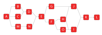
The complexity involved in an analytical solution can be best illustrated by looking at the simple complex system with 15 components, as shown in Figure " An RBD of a complex system".

Fig 5.1 An RBD of a complex system.

The system reliability for this system (computed using BlockSim) is shown next. The first solution is provided using BlockSim's symbolic solution. In symbolic mode, BlockSim breaks the equation into segments, identified by tokens, that need to be substituted into the final system equation for a complete solution. This creates algebraic solutions that are more compact than if the substitutions were made.

[math]\displaystyle{ \begin{align} {{R}_{System}}= & D2\cdot D3\cdot {{R}_{L}} \\ D3= & +{{R}_{K}}\cdot IK \\ IK= & +{{R}_{I}}\cdot {{R}_{J}}\cdot {{R}_{O}}\cdot {{R}_{G}}\cdot {{R}_{F}}\cdot {{R}_{H}}-{{R}_{I}}\cdot {{R}_{J}}\cdot {{R}_{O}}\cdot {{R}_{G}}\cdot {{R}_{F}} \\ & -{{R}_{I}}\cdot {{R}_{J}}\cdot {{R}_{F}}\cdot {{R}_{H}}-{{R}_{I}}\cdot {{R}_{O}}\cdot {{R}_{F}}\cdot {{R}_{H}} \\ & -{{R}_{J}}\cdot {{R}_{G}}\cdot {{R}_{F}}\cdot {{R}_{H}}+{{R}_{I}}\cdot {{R}_{O}}\cdot {{R}_{F}} \\ & +{{R}_{I}}\cdot {{R}_{F}}\cdot {{R}_{H}}+{{R}_{J}}\cdot {{R}_{F}}\cdot {{R}_{H}}+{{R}_{J}}\cdot {{R}_{G}} \\ D2 = & +{{R}_{A}}\cdot {{R}_{E}}\cdot IE \\ IE = & -D1\cdot {{R}_{M}}\cdot {{R}_{N}}+{{R}_{M}}\cdot {{R}_{N}}+D1 \\ D1 = & +{{R}_{D}}\cdot ID \\ ID = & -{{R}_{B}}\cdot {{R}_{C}}+{{R}_{B}}+{{R}_{C}} \end{align} }[/math]

Substituting the terms yields:

[math]\displaystyle{ \begin{align} {{R}_{System}}= & {{R}_{A}}\cdot {{R}_{E}}\cdot {{R}_{L}}\cdot {{R}_{K}} \\ & \cdot \{({{R}_{D}}\cdot {{R}_{B}}\cdot {{R}_{C}}+{{R}_{B}}+{{R}_{C}})\cdot {{R}_{M}}\cdot {{R}_{N}} \\ & +{{R}_{M}}\cdot {{R}_{N}}-{{R}_{D}}\cdot {{R}_{B}}\cdot {{R}_{C}}+{{R}_{B}}+{{R}_{C}}\} \\ & \cdot \{{{R}_{I}}\cdot {{R}_{J}}\cdot {{R}_{O}}\cdot {{R}_{G}}\cdot {{R}_{F}}\cdot {{R}_{H}}-{{R}_{I}}\cdot {{R}_{J}}\cdot {{R}_{O}}\cdot {{R}_{G}}\cdot {{R}_{F}} \\ & -{{R}_{I}}\cdot {{R}_{J}}\cdot {{R}_{F}}\cdot {{R}_{H}}-{{R}_{I}}\cdot {{R}_{O}}\cdot {{R}_{F}}\cdot {{R}_{H}} \\ & -{{R}_{J}}\cdot {{R}_{G}}\cdot {{R}_{F}}\cdot {{R}_{H}}+{{R}_{I}}\cdot {{R}_{O}}\cdot {{R}_{F}} \\ & +{{R}_{I}}\cdot {{R}_{F}}\cdot {{R}_{H}}+{{R}_{J}}\cdot {{R}_{F}}\cdot {{R}_{H}}+{{R}_{J}}\cdot {{R}_{G}}\} \end{align} }[/math]

BlockSim's automatic algebraic simplification would yield the following format for the above solution:

[math]\displaystyle{ \begin{align} {{R}_{System}}= & (({{R}_{A}}\cdot {{R}_{E}}(-({{R}_{D}}(-{{R}_{B}}\cdot {{R}_{C}}+{{R}_{B}}+{{R}_{C}})){{R}_{M}}\cdot {{R}_{N}} \\ & +{{R}_{M}}\cdot {{R}_{N}} \\ & +({{R}_{D}}(-{{R}_{B}}\cdot {{R}_{C}}+{{R}_{B}}+{{R}_{C}})))) \\ & ({{R}_{K}}({{R}_{I}}\cdot {{R}_{J}}\cdot {{R}_{O}}\cdot {{R}_{G}}\cdot {{R}_{F}}\cdot {{R}_{H}} \\ & -{{R}_{I}}\cdot {{R}_{J}}\cdot {{R}_{O}}\cdot {{R}_{G}}\cdot {{R}_{F}}-{{R}_{I}}\cdot {{R}_{J}}\cdot {{R}_{F}}\cdot {{R}_{H}} \\ & -{{R}_{I}}\cdot {{R}_{O}}\cdot {{R}_{F}}\cdot {{R}_{H}}-{{R}_{J}}\cdot {{R}_{G}}\cdot {{R}_{F}}\cdot {{R}_{H}} \\ & +RI\cdot {{R}_{O}}\cdot {{R}_{F}} \\ & +{{R}_{I}}\cdot {{R}_{F}}\cdot {{R}_{H}}+{{R}_{J}}\cdot {{R}_{F}}\cdot {{R}_{H}}+{{R}_{J}}\cdot {{R}_{G}})){{R}_{L}}) \ (eqn 2) \end{align} }[/math]

In this equation, each [math]\displaystyle{ {{R}_{i}} }[/math] represents the reliability function of a block. For example, if [math]\displaystyle{ {{R}_{A}} }[/math] has a Weibull distribution, then each [math]\displaystyle{ {{R}_{A}}(t)={{e}^{-{{\left( \tfrac{t}{{{\eta }_{A}}} \right)}^{{{\beta }_{A}}}}}} }[/math] and so forth. Substitution of each component's reliability function in the last [math]\displaystyle{ {{R}_{System}} }[/math] equation above will result in an analytical expression for the system reliability as a function of time, or [math]\displaystyle{ {{R}_{s}}(t) }[/math] , which is the same as [math]\displaystyle{ (1-cd{{f}_{System}}). }[/math]

Obtaining Other Functions of Interest

Once the system reliability equation (or the cumulative density function, [math]\displaystyle{ cdf }[/math] ) has been determined, other functions and metrics of interest can be derived.
Consider the following simple system:

Fig 5.2 Simple two-component system.

Furthermore, assume that component 1 follows an exponential distribution with a mean of 10,000 ([math]\displaystyle{ \mu =10,000, }[/math] [math]\displaystyle{ \lambda =1/10,000) }[/math] and component 2 follows a Weibull distribution with [math]\displaystyle{ \beta =6 }[/math] and [math]\displaystyle{ \eta =10,000 }[/math] . The reliability equation of this system is:

[math]\displaystyle{ \begin{align} {{R}_{S}}(t)= & {{R}_{1}}(t)\cdot {{R}_{2}}(t) \\ = & {{e}^{-\lambda t}}\cdot {{e}^{-{{\left( \tfrac{t}{\eta } \right)}^{\beta }}}} \\ = & {{e}^{-\tfrac{1}{10,000}t}}\cdot {{e}^{-{{\left( \tfrac{t}{10,000} \right)}^{6}}}} \ (eqn 3) \end{align} }[/math]

The system [math]\displaystyle{ cdf }[/math] is:

[math]\displaystyle{ \begin{align} {{F}_{S}}(t)= & 1-({{R}_{1}}(t)\cdot {{R}_{2}}(t)) \\ = & 1-\left( {{e}^{-\lambda t}}\cdot {{e}^{-{{\left( \tfrac{t}{\eta } \right)}^{\beta }}}} \right) \\ = & 1-\left( {{e}^{-\tfrac{1}{10,000}t}}\cdot {{e}^{-{{\left( \tfrac{t}{10,000} \right)}^{6}}}} \right) \end{align} }[/math]

Template:Analytical system pdf

Conditional Reliability

Conditional reliability is the probability of a system successfully completing another mission following the successful completion of a previous mission. The time of the previous mission and the time for the mission to be undertaken must be taken into account for conditional reliability calculations. The system's conditional reliability function is given by:

[math]\displaystyle{ R(T,t)=\frac{R(T+t)}{R(T)} }[/math]

Equation above gives the reliability for a new mission of duration [math]\displaystyle{ t }[/math] having already accumulated [math]\displaystyle{ T }[/math] hours of operation up to the start of this new mission. The system is evaluated to assure that it will start the next mission successfully.
For the system in Figure "Simple two-component system.", the reliability for mission of [math]\displaystyle{ t=1,000 }[/math] hours, having an age of [math]\displaystyle{ T=500 }[/math] hours, is:

[math]\displaystyle{ \begin{align} {{R}_{S}}(T=500,t=1000)= & \frac{R(T+t)}{R(T)} \\ = & \frac{R(1500)}{R(500)} \\ = & \frac{{{e}^{-\tfrac{1500}{10,000}}}\cdot {{e}^{-{{\left( \tfrac{1500}{10,000} \right)}^{6}}}}}{{{e}^{-\tfrac{500}{10,000}t}}\cdot {{e}^{-{{\left( \tfrac{500}{10,000} \right)}^{6}}}}} \\ = & 0.9048=90.48% \end{align} }[/math]

Conditional Reliability for Components

Now in this formulation, it was assumed that the accumulated age was equivalent for both units. That is, both started life at zero and aged to 500. It is possible to consider an individual component that has already accumulated some age (used component) in the same formulation. To illustrate this, assume that component 2 started life with an age of T=100. Then the reliability equation of the system, as given in [math]\displaystyle{ {{R}_{S}}(t)= {{R}_{1}}(t)\cdot {{R}_{2}}(t) }[/math], would need to be modified to include a conditional term for 2, or:

[math]\displaystyle{ {{R}_{S}}(t)={{R}_{1}}(t)\cdot \frac{{{R}_{2}}({{T}_{2}}+t)}{{{R}_{2}}({{T}_{2}})} \ (eqn 7) }[/math]

In BlockSim, the start age input box may be used to specify a starting age greater than zero.

System Mean Life (Mean Time To Failure)

The mean life (or mean time to failure, MTTF) can be obtained by integrating the system reliability function from zero to infinity:

[math]\displaystyle{ MTTF=\int_{0}^{\infty }{{R}_{s}}\left( t \right)dt \ }[/math]

The mean time is a performance index and does not provide any information about the behavior of the failure distribution of the system.
For the system in Figure "Simple two-component system":

[math]\displaystyle{ \begin{align} MTTF= & \int_{0}^{\infty }\left( {{e}^{-\tfrac{1}{10,000}t}}\cdot {{e}^{-{{\left( \tfrac{t}{10,000} \right)}^{6}}}} \right)dt \\ = & 5978.9 \end{align} }[/math]

Warranty Period and BX Life

Sometimes it is desirable to know the time value associated with a certain reliability. Warranty periods are often calculated by determining what percentage of the failure population can be covered financially and estimating the time at which this portion of the population will fail. Similarly, engineering specifications may call for a certain BX life, which also represents a time period during which a certain proportion of the population will fail. For example, the B10 life is the time in which 10% of the population will fail. This is obtained by setting [math]\displaystyle{ {{R}_{S}}(t) }[/math] to the desired value and solving for [math]\displaystyle{ t. }[/math]
For the system in Figure "Simple two-component system":

[math]\displaystyle{ {{R}_{s}}\left( t \right)={{e}^{-\tfrac{1}{10,000}t}}\cdot {{e}^{-{{\left( \tfrac{t}{10,000} \right)}^{6}}}} }[/math]

To compute the time by which reliability would be equal to 90%, equation above is recast as follows and solved for [math]\displaystyle{ t. }[/math]

[math]\displaystyle{ 0.90={{e}^{-\tfrac{1}{10,000}t}}\cdot {{e}^{-{{\left( \tfrac{t}{10,000} \right)}^{6}}}} }[/math]

In this case, [math]\displaystyle{ t=1053.59 }[/math] . Equivalently, the B10 life for this system is also [math]\displaystyle{ 1053.59 }[/math] . Except for some trivial cases, a closed form solution for [math]\displaystyle{ t }[/math] cannot be obtained. Thus, it is necessary to solve for [math]\displaystyle{ t }[/math] using numerical methods. BlockSim uses numerical methods.

Example 1

Consider a system consisting of three exponential units in series with the following failure rates (in failures per hour): [math]\displaystyle{ {{\lambda }_{1}} }[/math] = 0.0002, [math]\displaystyle{ {{\lambda }_{2}} }[/math] = 0.0005 and [math]\displaystyle{ {{\lambda }_{3}} }[/math] = 0.0001.

• Obtain the reliability equation for the system.

• What is the reliability of the system after 150 hours of operation?

• Obtain the system's [math]\displaystyle{ pdf. }[/math]

• Obtain the system's failure rate equation.

• What is the MTTF for the system?

• What should the warranty period be for a 90% reliability?

Solution to Example 1

• The analytical expression for the reliability of the system is given by:

[math]\displaystyle{ \begin{align} {{R}_{s}}(t)= & {{R}_{1}}(t)\cdot {{R}_{2}}(t)\cdot {{R}_{3}}(t) \\ = & {{e}^{-{{\lambda }_{1}}t}}\cdot {{e}^{-{{\lambda }_{2}}t}}\cdot {{e}^{-{{\lambda }_{1}}t}} \\ = & {{e}^{-({{\lambda }_{1}}+{{\lambda }_{2}}+{{\lambda }_{3}})t}} \end{align} }[/math]

At 150 hours of operation, the reliability of the system is:

[math]\displaystyle{ \begin{align} {{R}_{s}}(t)= & {{e}^{-(0.0002+0.0005+0.0001)150}} \\ = & 0.8869\text{ or }88.69% \end{align} }[/math]

• In order to obtain the system's [math]\displaystyle{ pdf }[/math] , the derivative of the reliability equation given in the first equation above is taken with respect to time, or:

[math]\displaystyle{ \begin{align} {{f}_{s}}(t)= & -\frac{d[{{R}_{s}}(t)]}{dt} \\ = & -\frac{d\left[ {{e}^{-({{\lambda }_{1}}+{{\lambda }_{2}}+{{\lambda }_{3}})t}} \right]}{dt} \\ = & ({{\lambda }_{1}}+{{\lambda }_{2}}+{{\lambda }_{3}})\cdot {{e}^{-({{\lambda }_{1}}+{{\lambda }_{2}}+{{\lambda }_{3}})t}} \end{align} }[/math]

• The system's failure rate can now be obtained simply by dividing the system's [math]\displaystyle{ pdf }[/math] given in the equation above by the system's reliability function given in the first equation above, and:

[math]\displaystyle{ \begin{align} {{\lambda }_{s}}\left( t \right)= & \frac{{{f}_{s}}\left( t \right)}{{{R}_{s}}\left( t \right)} \\ = & \frac{({{\lambda }_{1}}+{{\lambda }_{2}}+{{\lambda }_{3}})\cdot {{e}^{-({{\lambda }_{1}}+{{\lambda }_{2}}+{{\lambda }_{3}})t}}}{{{e}^{-({{\lambda }_{1}}+{{\lambda }_{2}}+{{\lambda }_{3}})t}}} \\ = & ({{\lambda }_{1}}+{{\lambda }_{2}}+{{\lambda }_{3}}) \\ = & 0.0008\text{ }fr/hr \end{align} }[/math]

• Combining [math]\displaystyle{ MTTF=\int_{0}^{\infty }{{R}_{s}}\left( t \right)dt \ }[/math] and the first equation above, the system's MTTF can be obtained:

[math]\displaystyle{ \begin{align} MTTF= & \int_{0}^{\infty }{{R}_{s}}\left( t \right)dt \\ = & \int_{0}^{\infty }{{e}^{-({{\lambda }_{1}}+{{\lambda }_{2}}+{{\lambda }_{3}})t}}dt \\ = & \frac{1}{({{\lambda }_{1}}+{{\lambda }_{2}}+{{\lambda }_{3}})} \\ = & 1250\text{ }hr \end{align} }[/math]

• Solving the first equation above with respect to time will yield the corresponding warranty period for a 90% reliability. In this case, the system reliability equation is simple and a closed form solution exists. The warranty time can now be found by solving:

[math]\displaystyle{ \begin{align} t= & -\frac{\ln (R)}{{{\lambda }_{1}}+{{\lambda }_{2}}+{{\lambda }_{3}}} \\ = & -\frac{\ln (0.9)}{0.0008} \\ = & 131.7\text{ }hr \end{align} }[/math]

Thus, the warranty period should be 132 hours.

Example 2

Consider the system shown in Figure "Complex bridge system in Example 2".

Fig 5.5 Complex bridge system in Example 2.

Components [math]\displaystyle{ A }[/math] through [math]\displaystyle{ E }[/math] are Weibull distributed with [math]\displaystyle{ \beta =1.2 }[/math] and [math]\displaystyle{ \eta =1230 }[/math] hours. The starting and ending blocks cannot fail.
Determine the following:

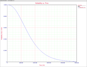
• The reliability equation for the system and its corresponding plot.

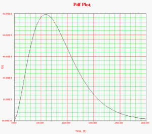
• The system's [math]\displaystyle{ pdf }[/math] and its corresponding plot.

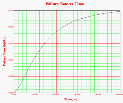
• The system's failure rate equation and the corresponding plot.

• The [math]\displaystyle{ MTTF }[/math] .

• The warranty time for a 90% reliability.

• The reliability for a 200-hour mission, if it is known that the system has already successfully operated for 200 hours.

Solution

The first step is to obtain the reliability function for the system. The methods described in the previous chapter can be employed, such as the event space or path-tracing methods. Using BlockSim, the following reliability equation is obtained:

[math]\displaystyle{ \begin{align} {{R}_{s}}(t)= & ({{R}_{Start}}\cdot {{R}_{End}}(2{{R}_{A}}\cdot {{R}_{D}}\cdot {{R}_{C}}\cdot {{R}_{B}}\cdot {{R}_{E}} \\ & -{{R}_{A}}\cdot {{R}_{D}}\cdot {{R}_{C}}\cdot {{R}_{B}}-{{R}_{A}}\cdot {{R}_{D}}\cdot {{R}_{C}}\cdot {{R}_{E}} \\ & -{{R}_{A}}\cdot {{R}_{D}}\cdot {{R}_{B}}\cdot {{R}_{E}}-{{R}_{A}}\cdot {{R}_{C}}\cdot {{R}_{B}}\cdot {{R}_{E}} \\ & -{{R}_{D}}\cdot {{R}_{C}}\cdot {{R}_{B}}\cdot {{R}_{E}}+{{R}_{A}}\cdot {{R}_{C}}\cdot {{R}_{E}} \\ & +{{R}_{D}}\cdot {{R}_{C}}\cdot {{R}_{B}}+{{R}_{A}}\cdot {{R}_{D}}+{{R}_{B}}\cdot {{R}_{E}})) \end{align} }[/math]

Note that since the starting and ending blocks cannot fail, [math]\displaystyle{ {{R}_{Start}}=1 }[/math] and [math]\displaystyle{ {{R}_{End}}=1, }[/math] equation above can be reduced to:

[math]\displaystyle{ \begin{align} {{R}_{s}}(t)= & 2\cdot {{R}_{A}}\cdot {{R}_{D}}\cdot {{R}_{C}}\cdot {{R}_{B}}\cdot {{R}_{E}} \\ & -{{R}_{A}}\cdot {{R}_{D}}\cdot {{R}_{C}}\cdot {{R}_{B}}-{{R}_{A}}\cdot {{R}_{D}}\cdot {{R}_{C}}\cdot {{R}_{E}} \\ & -{{R}_{A}}\cdot {{R}_{D}}\cdot {{R}_{B}}\cdot {{R}_{E}}-{{R}_{A}}\cdot {{R}_{C}}\cdot {{R}_{B}}\cdot {{R}_{E}} \\ & -{{R}_{D}}\cdot {{R}_{C}}\cdot {{R}_{B}}\cdot {{R}_{E}}+{{R}_{A}}\cdot {{R}_{C}}\cdot {{R}_{E}} \\ & +{{R}_{D}}\cdot {{R}_{C}}\cdot {{R}_{B}}+{{R}_{A}}\cdot {{R}_{D}}+{{R}_{B}}\cdot {{R}_{E}} \end{align} }[/math]

Where [math]\displaystyle{ {{R}_{A}} }[/math] is the reliability equation for Component A, or:

[math]\displaystyle{ {{R}_{A}}(t)={{e}^{-{{\left( \tfrac{t}{{{\eta }_{A}}} \right)}^{{{\beta }_{A}}}}}} }[/math]

[math]\displaystyle{ {{R}_{B}} }[/math] is the reliability equation for Component [math]\displaystyle{ B }[/math] , etc.

Since the components in this example are identical, the system reliability equation can be further reduced to:

[math]\displaystyle{ {{R}_{s}}(t)=2R{{(t)}^{2}}+2R{{(t)}^{3}}-5R{{(t)}^{4}}+2R{{(t)}^{5}} }[/math]

Or, in terms of the failure distribution:

[math]\displaystyle{ {{R}_{s}}(t)=2\cdot {{e}^{-2{{\left( \tfrac{t}{\eta } \right)}^{\beta }}}}+2\cdot {{e}^{-3{{\left( \tfrac{t}{\eta } \right)}^{\beta }}}}-5\cdot {{e}^{-4{{\left( \tfrac{t}{\eta } \right)}^{\beta }}}}+2\cdot {{e}^{-5{{\left( \tfrac{t}{\eta } \right)}^{\beta }}}} }[/math]

The corresponding plot is given in Figure "Reliability plot for the system".

Reliability plot for the system.

In order to obtain the system's [math]\displaystyle{ pdf }[/math] , the derivative of the reliability equation given above is taken with respect to time, resulting in:

[math]\displaystyle{ \begin{align} {{f}_{s}}(t)= & 4\cdot \frac{\beta }{\eta }{{\left( \frac{t}{\eta } \right)}^{\beta -1}}{{e}^{-2{{\left( \tfrac{t}{\eta } \right)}^{\beta }}}}+6\cdot \frac{\beta }{\eta }{{\left( \frac{t}{\eta } \right)}^{\beta -1}}{{e}^{-3{{\left( \tfrac{t}{\eta } \right)}^{\beta }}}} \\ & -20\cdot \frac{\beta }{\eta }{{\left( \frac{t}{\eta } \right)}^{\beta -1}}{{e}^{-4{{\left( \tfrac{t}{\eta } \right)}^{\beta }}}}+10\cdot \frac{\beta }{\eta }{{\left( \frac{t}{\eta } \right)}^{\beta -1}}{{e}^{-5{{\left( \tfrac{t}{\eta } \right)}^{\beta }}}} \end{align} }[/math]

The [math]\displaystyle{ pdf }[/math] can now be plotted for different time values, [math]\displaystyle{ t }[/math] , as shown in Figure "pdf plot for the system".

The system's failure rate can now be obtained by dividing the system's [math]\displaystyle{ pdf }[/math] given in equation above by the system's reliability function given in [math]\displaystyle{ {{R}_{s}}(t)=2\cdot {{e}^{-2{{\left( \tfrac{t}{\eta } \right)}^{\beta }}}}+2\cdot {{e}^{-3{{\left( \tfrac{t}{\eta } \right)}^{\beta }}}}-5\cdot {{e}^{-4{{\left( \tfrac{t}{\eta } \right)}^{\beta }}}}+2\cdot {{e}^{-5{{\left( \tfrac{t}{\eta } \right)}^{\beta }}}} }[/math], or:

[math]\displaystyle{ \begin{align} {{\lambda }_{s}}(t)= & \frac{4\cdot \tfrac{\beta }{\eta }{{\left( \tfrac{t}{\eta } \right)}^{\beta -1}}{{e}^{-2{{\left( \tfrac{t}{\eta } \right)}^{\beta }}}}+6\cdot \tfrac{\beta }{\eta }{{\left( \tfrac{t}{\eta } \right)}^{\beta -1}}{{e}^{-3{{\left( \tfrac{t}{\eta } \right)}^{\beta }}}}}{2\cdot {{e}^{-2{{\left( \tfrac{t}{\eta } \right)}^{\beta }}}}+2\cdot {{e}^{-3{{\left( \tfrac{t}{\eta } \right)}^{\beta }}}}-5\cdot {{e}^{-4{{\left( \tfrac{t}{\eta } \right)}^{\beta }}}}+2\cdot {{e}^{-5{{\left( \tfrac{t}{\eta } \right)}^{\beta }}}}} \\ & +\frac{-20\cdot \tfrac{\beta }{\eta }{{\left( \tfrac{t}{\eta } \right)}^{\beta -1}}{{e}^{-4{{\left( \tfrac{t}{\eta } \right)}^{\beta }}}}+10\cdot \tfrac{\beta }{\eta }{{\left( \tfrac{t}{\eta } \right)}^{\beta -1}}{{e}^{-5{{\left( \tfrac{t}{\eta } \right)}^{\beta }}}}}{2\cdot {{e}^{-2{{\left( \tfrac{t}{\eta } \right)}^{\beta }}}}+2\cdot {{e}^{-3{{\left( \tfrac{t}{\eta } \right)}^{\beta }}}}-5\cdot {{e}^{-4{{\left( \tfrac{t}{\eta } \right)}^{\beta }}}}+2\cdot {{e}^{-5{{\left( \tfrac{t}{\eta } \right)}^{\beta }}}}} \end{align} }[/math]

The corresponding plot is given in Figure "Failure rate for the system".

pdf plot for the system.

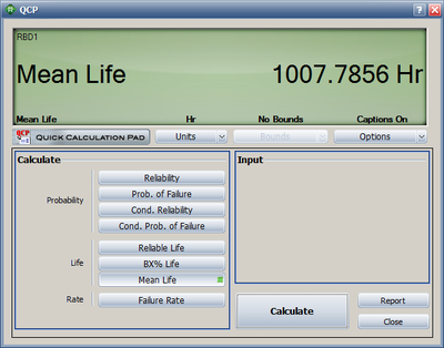
The [math]\displaystyle{ MTTF }[/math] of the system is obtained by integrating the system's reliability function given by [math]\displaystyle{ {{R}_{s}}(t)=2\cdot {{e}^{-2{{\left( \tfrac{t}{\eta } \right)}^{\beta }}}}+2\cdot {{e}^{-3{{\left( \tfrac{t}{\eta } \right)}^{\beta }}}}-5\cdot {{e}^{-4{{\left( \tfrac{t}{\eta } \right)}^{\beta }}}}+2\cdot {{e}^{-5{{\left( \tfrac{t}{\eta } \right)}^{\beta }}}} }[/math] from time zero to infinity, as given by [math]\displaystyle{ MTTF=\int_{0}^{\infty }{{R}_{s}}\left( t \right)dt \ }[/math]. Using BlockSim's Analytical QCP, an [math]\displaystyle{ MTTF }[/math] of 1007.8 hours is calculated, as shown in Figure "MTTF of the system".

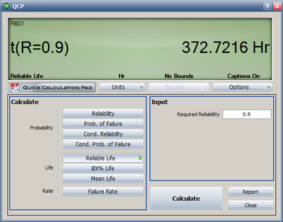
The warranty time can be obtained by solving [math]\displaystyle{ {{R}_{s}}(t) }[/math] with respect to time for a system reliability [math]\displaystyle{ {{R}_{s}}=0.9 }[/math] . Using the Analytical QCP and selecting the
Warranty Time option, a time of 372.72 hours is obtained, as shown in Figure "Time at which R=0.9 or 90% for the system".

Failure rate for the system.

MTTF of the system.

Time at which R=0.9 or 90% for the system.

Conditional reliability calculation for the system.

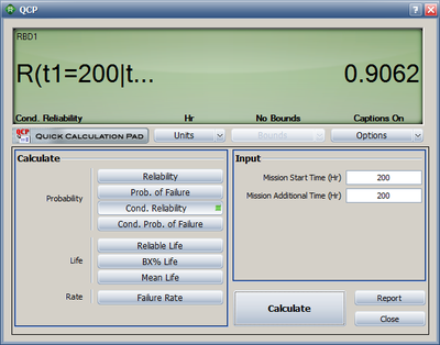
Lastly, the conditional reliability can be obtained using [math]\displaystyle{ R(T,t)=\frac{R(T+t)}{R(T)} }[/math] and [math]\displaystyle{ {{R}_{s}}(t)=2\cdot {{e}^{-2{{\left( \tfrac{t}{\eta } \right)}^{\beta }}}}+2\cdot {{e}^{-3{{\left( \tfrac{t}{\eta } \right)}^{\beta }}}}-5\cdot {{e}^{-4{{\left( \tfrac{t}{\eta } \right)}^{\beta }}}}+2\cdot {{e}^{-5{{\left( \tfrac{t}{\eta } \right)}^{\beta }}}} }[/math], or:

[math]\displaystyle{ \begin{align} R(200,200)= & \frac{R(400)}{R(200)} \\ = & \frac{0.883825}{0.975321} \\ = & 0.906189 \end{align} }[/math]

This can be calculated using BlockSim's Analytical QCP, as shown in Figure "Conditional reliability calculation for the system".

Approximating the System CDF

In many cases, it is valuable to fit a distribution that represents the system's times-to-failure. This can be useful when the system is part of a larger assembly and may be used for repeated calculations or in calculations for other systems. In cases such as this, it can be useful to characterize the system's behavior by fitting a distribution to the overall system and calculating parameters for this distribution. This is equivalent to fitting a single distribution to describe [math]\displaystyle{ {{R}_{S}}(t }[/math] ). In essence, it is like reducing the entire system to a component in order to simplify calculations.
For the system in Figure below:

Simple two-component system.

[math]\displaystyle{ {{R}_{S}}(t)={{e}^{-\tfrac{1}{10,000}t}}\cdot {{e}^{-{{\left( \tfrac{t}{10,000} \right)}^{6}}}} }[/math]

To compute an approximate reliability function for this system, [math]\displaystyle{ {{R}_{A}}(t)\simeq {{R}_{S}}(t) }[/math] , one would compute [math]\displaystyle{ n }[/math] pairs of reliability and time values and then fit a single distribution to the data, or:

[math]\displaystyle{ \begin{align} {{R}_{S}}(t= & 10,396.7)=10% \\ {{R}_{S}}(t= & 9,361.9)=20% \\ & ... \\ {{R}_{S}}(t= & 1,053.6)=90% \end{align} }[/math]

A single distribution, [math]\displaystyle{ {{R}_{A}}(t) }[/math] , that approximates [math]\displaystyle{ {{R}_{S}}(t) }[/math] can now be computed from these pairs using life data analysis methods. If using the Weibull++ software, one would enter the values as free form data.

Example 3

Compute a single Weibull distribution approximation for the system in Example 2.

Solution to Example 3

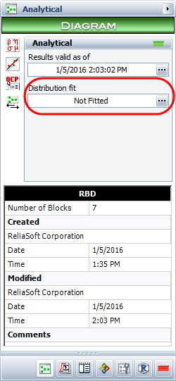
The system in the previous example, shown in Figure "Complex bridge system in Example 2", can be approximated by use of a 2-parameter Weibull distribution with [math]\displaystyle{ \beta =2.02109 }[/math] and [math]\displaystyle{ \eta =1123.51 }[/math] . In BlockSim, this is accomplished by representing the entire system as one distribution by going to the Distribution Fit window Figure " Representing a system with a distribution".

Fig 5.12 Representing a system with a distribution.

Fig 5.13 Distribution Fitting window.

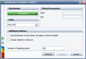
by clicking the Distribution Fit Window, the Distribution Estimator window will appear (Figure "Distribution Fitting window").
In this window you can select a distribution to represent the data. BlockSim will then generate a number of system failure times based on the system's reliability function. The system's reliability function can be used to solve for a time value associated with that unreliability value. The distribution of the generated time values can then be fitted to a probability distribution function.

Consider a value of [math]\displaystyle{ F(t)=0.11 }[/math] . Using the system's reliability equation and solving for time, the corresponding time-to-failure for a 0.11 unreliability can be calculated.
For the system of Example 2, the time for a 0.11 unreliability is 389.786 hours.
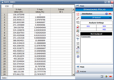
When enough points have been generated, the selected distribution will be fitted to this data set and the distribution's parameters will be returned. In addition, if ReliaSoft's Weibull++ is installed, the generated data can be viewed/analyzed using a Weibull++ instance, as shown in Figure "Using Weibull++ to calculate distribution parameters".

Fig 5.14 Using Weibull++ to calculate distribution parameters.

It is recommended that the analyst examine the fit to ascertain the applicability of the approximation.

Duty Cycle

Components of a system may not operate continuously during a system's mission, or may be subjected to loads greater or lesser than the rated loads during system operation. To model this, a factor called the Duty Cycle ( [math]\displaystyle{ {{d}_{c}} }[/math] ) is used. The duty cycle may also be used to account for changes in environmental stress, such as temperature changes, that may effect the operation of a component. The duty cycle is a positive value, with a default value of 1 representing continuous operation at rated load, and any values other than 1 representing other load values with respect to the rated load value (or total operating time). A duty cycle value higher than 1 indicates a load in excess of the rated value. A duty cycle value lower than 1 indicates that the component is operating at a load lower than the rated load or not operating continuously during the system's mission. For instance, a duty cycle of 0.5 may be used for a component that operates only half of the time during the system's mission.
The reliability metrics for a component with a duty cycle are calculated as follows. Let [math]\displaystyle{ {{d}_{c}} }[/math] represent the duty cycle during a particular mission of the component, [math]\displaystyle{ t }[/math] represent the mission time and [math]\displaystyle{ {t}' }[/math] represent the accumulated age. Then:

[math]\displaystyle{ {t}'={{d}_{c}}\times t }[/math]

The reliability equation for the component is:

[math]\displaystyle{ R({t}')=R({{d}_{c}}\times t) }[/math]

The component pdf is:

[math]\displaystyle{ f({t}')=-\frac{d(R({t}'))}{dt}=-\frac{d(R({{d}_{c}}\times t))}{dt}={{d}_{c}}f({{d}_{c}}\times t) }[/math]

The failure rate of the component is:

[math]\displaystyle{ \lambda ({t}')=\frac{f({t}')}{R({t}')}=\frac{{{d}_{c}}f({{d}_{c}}\times t)}{R({{d}_{c}}\times t)}={{d}_{c}}\lambda ({{d}_{c}}\times t) }[/math]

Example 4

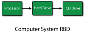
Consider a computer system with three components: a processor, a hard drive and a CD drive in series as shown next. Assume that all three components follow a Weibull failure distribution with the parameters [math]\displaystyle{ {{\beta }_{1}}=1.5 }[/math] and [math]\displaystyle{ {{\eta }_{1}}=5000 }[/math] for the processor, [math]\displaystyle{ {{\beta }_{2}}=2.5 }[/math] and [math]\displaystyle{ {{\eta }_{2}}=3000 }[/math] for the hard drive, and [math]\displaystyle{ {{\beta }_{3}}=2 }[/math] and [math]\displaystyle{ {{\eta }_{3}}=4000 }[/math] for the CD drive. Determine the reliability of the computer system after one year (365 days) of operation, assuming that the CD drive is used only 30% of the time.

Solution to Example 4

The reliability of the processor after 365 days of operation is given by:

[math]\displaystyle{ \begin{align} {{R}_{processor}}(365)= & {{e}^{-{{\left( \tfrac{365}{{{\eta }_{1}}} \right)}^{{{\beta }_{1}}}}}} \\ = & {{e}^{-{{\left( \tfrac{365}{5000} \right)}^{1.5}}}} \\ = & 0.9805\text{ or }98.05% \end{align} }[/math]

The reliability of the hard drive after 365 days of operation is given by:

[math]\displaystyle{ \begin{align} {{R}_{harddrive}}(365)= & {{e}^{-{{\left( \tfrac{365}{{{\eta }_{2}}} \right)}^{{{\beta }_{2}}}}}} \\ = & {{e}^{-{{\left( \tfrac{365}{3000} \right)}^{2.5}}}} \\ = & 0.9948\text{ or }99.48% \end{align} }[/math]

The reliability of the CD drive after 365 days of operation (taking into account the 30% operation using a duty cycle of 0.3) is given by:

[math]\displaystyle{ \begin{align} {{R}_{CDdrive}}(365)= & {{e}^{-{{\left( \tfrac{{{d}_{c}}\times 365}{{{\eta }_{3}}} \right)}^{{{\beta }_{3}}}}}} \\ = & {{e}^{-{{\left( \tfrac{0.3\times 365}{4000} \right)}^{2}}}} \\ = & 0.9993\text{ or }99.93% \end{align} }[/math]

Fig 5.15 Result for the computer system reliability.

Thus the reliability of the computer system after 365 days of operation is:

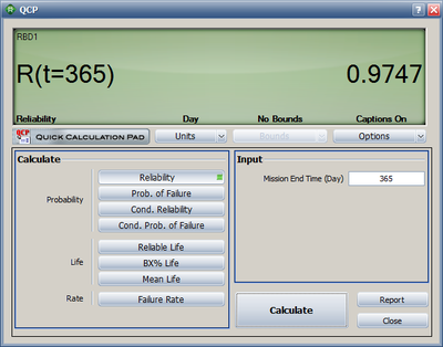
[math]\displaystyle{ \begin{align} {{R}_{s}}(365)= & {{R}_{processor}}(365)\cdot {{R}_{harddrive}}(365)\cdot {{R}_{CDdrive}}(365) \\ = & 0.9805\cdot 0.9948\cdot 0.9993 \\ = & 0.9747\text{ or }97.47% \end{align} }[/math]

This result can be obtained in BlockSim as shown in Figure "Result for the computer system reliability".

Load Sharing

As presented in earlier chapters, a reliability block diagram (RBD) allows you to graphically represent how the components within a system are reliability-wise connected. In most cases, independence is assumed across the components within the system. For example, the failure of component A does not affect the failure of component B. However, if a system consists of components that are sharing a load, then the assumption of independence no longer holds true.

If one component fails, then the component(s) that are still operating will have to assume the failed unit's portion of the load. Therefore, the reliabilities of the surviving unit(s) will change. Calculating the system reliability is no longer an easy proposition. In the case of load sharing components, the change of the failure distributions of the surviving components must be known in order to determine the system's reliability.

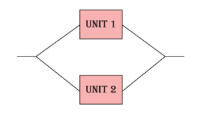
To illustrate this, consider the a system of two units connected reliability-wise in parallel (Figure "Two units connected reliability-wise in parallel").

Two units connected reliability-wise in parallel.

Assume that the units must supply an output of 8 volts and that if both units are operational, each unit is to supply 50% of the total output. If one of the units fails, then the surviving unit supplies 100%. Furthermore, assume that having to supply the entire load has a negative impact on the reliability characteristics of the surviving unit. Since the reliability characteristics of the unit change based on whether both or only one is operating, a life distribution along with a life-stress relationship (as discussed in Brief Introduction to Life-Stress Relationships) will be needed to model each component.

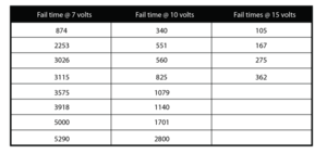
To illustrate the steps needed, we will create the model starting from raw data. Assume that a total of 20 units were tested to failure at 7, 10 and 15 volts. The test data set is presented in the next table.

For this example, Units 1 and 2 are the same component. Therefore, only one set of data was collected. However, it is possible that the load sharing components in a system may not be the same. If that were the case, data would need to be collected for each component.

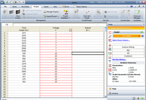
The data set in Table 1 was analyzed using ReliaSoft's ALTA software (as shown in Figure "Using ALTA to calculate component parameters") with the Inverse Power Law as the underlying life-stress relationship and Weibull as the life distribution.

The estimated model parameters, [math]\displaystyle{ \beta }[/math] , [math]\displaystyle{ K }[/math] and [math]\displaystyle{ n }[/math] , are shown next.

[math]\displaystyle{ \begin{align} \beta = & 1.9239 \\ K= & 3.2387\times {{10}^{-7}} \\ n= & 3.4226 \end{align} }[/math]

Or:

[math]\displaystyle{ \begin{align} {{R}_{1}}(t,{{S}_{1}})= & {{e}^{-{{\left( KS_{1}^{n}t \right)}^{\beta }}}} \\ = & {{e}^{-{{\left( 3.2387\times {{10}^{-7}}S_{1}^{3.4226}t \right)}^{1.9239}}}} \ \end{align} }[/math].

[math]\displaystyle{ {{f}_{1}}(t,{{S}_{1}})=\beta KS_{1}^{n}{{\left( KS_{1}^{n}t \right)}^{\beta -1}}{{e}^{-{{\left( KS_{1}^{n}t \right)}^{\beta }}}} \ (eqn 21 ) }[/math]

And for this case:

[math]\displaystyle{ \begin{align} {{R}_{1}}(t,{{S}_{1}})= & {{R}_{2}}(t,{{S}_{2}}) \\ {{f}_{1}}(t,{{S}_{1}})= & {{f}_{2}}(t,{{S}_{2}}) \end{align} }[/math]

Using ALTA to calculate component parameters.

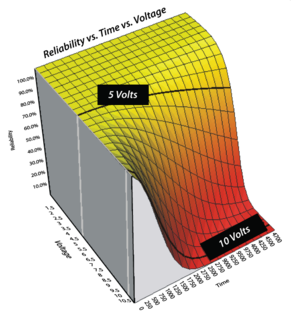
Figure "Reliability curves for different voltage output conditions" shows a plot of [math]\displaystyle{ {{R}_{1}}(t,{{S}_{1}})={{e}^{-{{\left( KS_{1}^{n}t \right)}^{\beta }}}} = {{e}^{-{{\left( 3.2387\times {{10}^{-7}}S_{1}^{3.4226}t \right)}^{1.9239}}}}\ }[/math].

Now that the failure properties have been determined using the test data, the reliability of the system at some time, [math]\displaystyle{ t }[/math] , can be calculated using the following equation:

[math]\displaystyle{ \begin{align} R(t,S)= & {{R}_{1}}(t,{{S}_{1}})\cdot {{R}_{2}}(t,{{S}_{2}}) \\ & +\underset{o}{\overset{t}{\mathop \int }}\,{{f}_{1}}\left( x,{{S}_{1}} \right)\cdot {{R}_{2}}(x,{{S}_{2}})\cdot \left( \frac{{{R}_{2}}({{t}_{1e}}+(t-x),S)}{{{R}_{2}}({{t}_{1e}},S)} \right)dx \\ & +\underset{o}{\overset{t}{\mathop \int }}\,{{f}_{2}}\left( x,{{S}_{2}} \right)\cdot {{R}_{1}}(x,{{S}_{1}})\cdot \left( \frac{{{R}_{1}}({{t}_{2e}}+(t-x),S)}{{{R}_{1}}({{t}_{2e}},S)} \right)dx \end{align} }[/math]

Where:

[math]\displaystyle{ \begin{align} {{S}_{1}}= & {{P}_{1}}S \\ {{S}_{2}}= & {{P}_{2}}S \end{align} }[/math]

Reliability curves for different voltage output conditions.

Illustrating [math]\displaystyle{ {{t}_{e}} }[/math]

And:

• [math]\displaystyle{ S }[/math] is the total load (or required output).

• [math]\displaystyle{ {{P}_{1}} }[/math] and [math]\displaystyle{ {{P}_{2}} }[/math] are the portion of the total load that each unit supports when both units are operational. In this case, [math]\displaystyle{ {{P}_{1}}={{P}_{2}}=0.5=50%. }[/math]

• [math]\displaystyle{ {{S}_{1}} }[/math] and [math]\displaystyle{ {{S}_{2}} }[/math] represent the portions of the load that Unit 1 and Unit 2 must support when both units are operational.

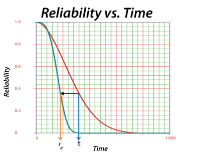
• [math]\displaystyle{ {{t}_{{{1}_{e}}}} }[/math] is the equivalent operating time for Unit 1 if it had been operating at [math]\displaystyle{ S }[/math] instead of [math]\displaystyle{ {{S}_{1}} }[/math] . A graphical representation of the equivalent time is shown in Figure 5.19, where the curve marked by L represents the low stress (load) and the curve marked by H represents the high stress (load).

[math]\displaystyle{ {{t}_{1e}} }[/math] can be calculated by:

[math]\displaystyle{ \begin{align} {{R}_{1}}(t)= & {{R}_{1}}({{t}_{1e}}) \\ {{e}^{-{{(tKS_{1}^{n})}^{\beta }}}}= & {{e}^{-{{({{t}_{1e}}K{{S}^{n}})}^{\beta }}}} \\ tS_{1}^{n}= & {{t}_{1e}}{{S}^{n}} \\ {{t}_{1e}}= & t{{\left( \frac{{{S}_{1}}}{S} \right)}^{n}},\text{ }{{S}_{1}}={{P}_{1}}S \\ \therefore & {{t}_{1e}}=tP_{1}^{n} \end{align} }[/math]

[math]\displaystyle{ {{t}_{2e}} }[/math] can be calculated the same way, or:

[math]\displaystyle{ \begin{align} {{R}_{2}}(t)= & {{R}_{2}}({{t}_{2e}}) \\ \therefore & {{t}_{2e}}=tP_{2}^{n} \end{align} }[/math]

In this example, the reliability equations for Unit 1 and Unit 2 are the same since they are the same type of component and demonstrate the same failure properties. In addition, the total output is divided equally between the two units (when both units are operating), so [math]\displaystyle{ {{t}_{1e}} }[/math] and [math]\displaystyle{ {{t}_{2e}} }[/math] will also be the same.
The next step is to determine the reliability of the system after 8,760 hours, [math]\displaystyle{ R(t=8,760) }[/math] . Using [math]\displaystyle{ \begin{align} R(t,S)= & {{R}_{1}}(t,{{S}_{1}})\cdot {{R}_{2}}(t,{{S}_{2}})+\underset{o}{\overset{t}{\mathop \int }}\,{{f}_{1}}\left( x,{{S}_{1}} \right)\cdot {{R}_{2}}(x,{{S}_{2}})\cdot \left( \frac{{{R}_{2}}({{t}_{1e}}+(t-x),S)}{{{R}_{2}}({{t}_{1e}},S)} \right)dx +\underset{o}{\overset{t}{\mathop \int }}\,{{f}_{2}}\left( x,{{S}_{2}} \right)\cdot {{R}_{1}}(x,{{S}_{1}})\cdot \left( \frac{{{R}_{1}}({{t}_{2e}}+(t-x),S)}{{{R}_{1}}({{t}_{2e}},S)} \right)dx \end{align} }[/math] the system reliability is found to be:

[math]\displaystyle{ \begin{align} R(t=8760)= & 0.8567 \\ = & 85.67% \end{align} }[/math]

Load Sharing in BlockSim

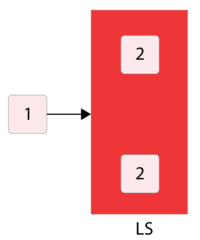
BlockSim uses this formulation when computing reliabilities of units in a load sharing configuration. When using the System Reliability Equation window, BlockSim returns a single token for the reliability of units in a load sharing configuration (as well as in the case of standby redundancy, discussed in the next section). As an example, consider the following RBD with Unit 1 in series with a container that includes two load sharing units.

BlockSim will return the system equation as:

[math]\displaystyle{ {{R}_{System}}=+{{R}_{LS}}\cdot {{R}_{1}} }[/math]

Where [math]\displaystyle{ {{R}_{LS}} }[/math] implies a form similar to Eqn. 22. BlockSim allows for [math]\displaystyle{ k }[/math] -out-of- [math]\displaystyle{ n }[/math] units in a load sharing configuration.

Example 5

A component has five possible failure modes, [math]\displaystyle{ A }[/math] , [math]\displaystyle{ {{B}_{A}} }[/math] , [math]\displaystyle{ {{B}_{B}} }[/math] , [math]\displaystyle{ {{B}_{C}} }[/math] and [math]\displaystyle{ C }[/math] , and the [math]\displaystyle{ B }[/math] modes are interdependent. The system will fail if mode [math]\displaystyle{ A }[/math] occurs, mode [math]\displaystyle{ C }[/math] occurs or two out of the three [math]\displaystyle{ B }[/math] modes occur.

Modes [math]\displaystyle{ A }[/math] and [math]\displaystyle{ C }[/math] each have a Weibull distribution, with a [math]\displaystyle{ \beta =2 }[/math] and [math]\displaystyle{ \eta =10,000 }[/math] and 15,000 respectively. Events [math]\displaystyle{ {{B}_{A}} }[/math] , [math]\displaystyle{ {{B}_{B}} }[/math] and [math]\displaystyle{ {{B}_{C}} }[/math] each have an exponential distribution with a mean of 10,000 hours.

If any [math]\displaystyle{ B }[/math] event occurs (i.e. [math]\displaystyle{ {{B}_{A}} }[/math] , [math]\displaystyle{ {{B}_{B}} }[/math] or [math]\displaystyle{ {{B}_{C}} }[/math] ), the remaining [math]\displaystyle{ B }[/math] events are more likely to occur. Specifically, the mean times of the remaining [math]\displaystyle{ B }[/math] events are halved. Determine the reliability at 1000 hours for this component.

Solution to Example 5

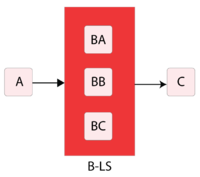
The first step is to create the RBD. Modes [math]\displaystyle{ A }[/math] , [math]\displaystyle{ C }[/math] and a load sharing container with the [math]\displaystyle{ {{B}_{i}} }[/math] modes must be drawn in series, as illustrated next.

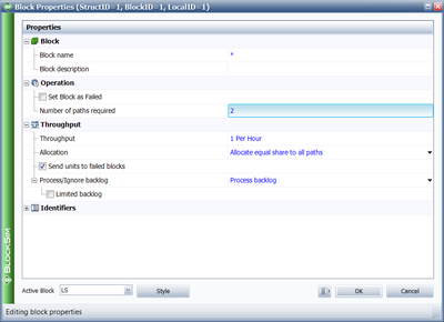
The next step is to define the properties for each block, including those for the container. Setting the failure distributions for modes [math]\displaystyle{ A }[/math] and [math]\displaystyle{ C }[/math] is simple. The more difficult part is setting the properties for the container and the contained blocks. Based on the problem statement, the [math]\displaystyle{ B }[/math] modes are in a 2-out-of-3 load sharing redundancy. When all three are working (i.e. when no [math]\displaystyle{ B }[/math] mode has occurred), each block has an exponential distribution with [math]\displaystyle{ \mu=10,000 }[/math]. If one [math]\displaystyle{ B }[/math] mode occurs, then the two surviving units have an exponential distribution with [math]\displaystyle{ \mu =5,000. }[/math]

Assume a Power Life-Stress relationship for the components. Then:

[math]\displaystyle{ \begin{align} {{\mu }_{1}}= & \frac{1}{KV_{1}^{n}} \ (eqn 23)\\ {{\mu }_{2}}= & \frac{1}{KV_{2}^{n}} \ (eqn 24) \end{align} }[/math]

Substituting [math]\displaystyle{ {{\mu }_{1}}=10,000 }[/math] and [math]\displaystyle{ {{V}_{1}}=1 }[/math] in Eqn. 23 and casting it in terms of [math]\displaystyle{ K }[/math] yields:

[math]\displaystyle{ \begin{align} 10,000= & \frac{1}{K} \ (eqn 25) \\ K = & \frac{1}{10,000}=0.0001 \end{align} }[/math]

Substituting [math]\displaystyle{ {{\mu }_{2}}=5,000 }[/math] , [math]\displaystyle{ {{V}_{2}}=1.5 }[/math] (because if one fails, then each survivor takes on an additional 0.5 units of load) and Eqn. 25 for [math]\displaystyle{ K }[/math] in Eqn.24 yields:

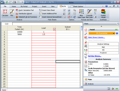
[math]\displaystyle{ \begin{align} 5,000= & \frac{1}{0.0001\cdot {{(1.5)}^{n}}} \\ 0.5= & {{(1.5)}^{-n}} \\ \ln (0.5)= & -n\ln (1.5) \\ n = & 1.7095 \end{align} }[/math]

This also could have been computed in ALTA, as shown in Figure "Calculation performed in ALTA".

The next step is to set the weight proportionality factor. This factor defines the portion of the load that the particular item carries while operating, as well as the load that shifts to the remaining units upon failure of the item. To illustrate, assume three units (1, 2 and 3) are in a load sharing container with weight proportionality factors of 1, 2 and 3 respectively (and a 1-out-of-3 requirement).

• Unit 1 carries [math]\displaystyle{ \left( \tfrac{1}{1+2+3} \right)=0.166 }[/math] or 16.6% of the total load.

• Unit 2 carries [math]\displaystyle{ \left( \tfrac{2}{1+2+3} \right)=0.333 }[/math] or 33.3% of the total load.

• Unit 3 carries [math]\displaystyle{ \left( \tfrac{3}{1+2+3} \right)=0.50 }[/math] or 50% of the total load.

The actual load on each unit then becomes the product of the entire load defined for the container times the portion carried by that unit. For example, if the container load is 100 lbs, then the portion assigned to Unit 1 will be [math]\displaystyle{ 100\cdot 0.166=16.6 }[/math] lbs.

In the current example, all units share the same load and thus have equal weight proportionality factors. Because these factors are relative, if the same number is used for all three items then the results will be the same. Thus, weight proportional factor is set equal to 1 for each item.

Calculation performed in ALTA.

Defining Weight Proportional Factor.

The last properties that need to be defined are the total load and the 2-out-of-3 redundancy. The total load is dependent on how the parameters were computed. In this case, total load was assumed to be 3 when the parameters were computed (i.e. the load per item was 1 when all worked and 1.5 when two worked). This is defined at the container level, as shown in Figure "Defining Weight Proportional Factor". When all of the parameters have been specified in BlockSim, the reliability at 1,000 hours can be determined. From the Analytical QCP, this is found to be 93.87%.

Standby Components

In the previous section, the case of a system with load sharing components was presented. This is a form of redundancy with dependent components. That is, the failure of one component affects the failure of the other(s). This section presents another form of redundancy: standby redundancy. In standby redundancy the redundant components are set to be under a lighter load condition (or no load) while not needed and under the operating load when they are activated.

In standby redundancy the components are set to have two states: an active state and a standby state. Components in standby redundancy have two failure distributions, one for each state. When in the standby state, they have a quiescent (or dormant) failure distribution and when operating, they have an active failure distribution.

In the case that both quiescent and active failure distributions are the same, the units are in a simple parallel configuration (also called a hot standby configuration). When the rate of failure of the standby component is lower in quiescent mode than in active mode, that is called a warm standby configuration. When the rate of failure of the standby component is zero in quiescent mode (i.e. the component cannot fail when in standby), that is called a cold standby configuration.

Simple Standby Configuration

Consider two components in a standby configuration. Component 1 is the active component with a Weibull failure distribution with parameters [math]\displaystyle{ \beta }[/math] = 1.5 and [math]\displaystyle{ \eta }[/math] = 1,000. Component 2 is the standby component. When Component 2 is operating, it also has a Weibull failure distribution with [math]\displaystyle{ \beta }[/math] = 1.5 and [math]\displaystyle{ \eta }[/math] = 1,000. Furthermore, assume the following cases for the quiescent distribution.

• Case 1: The quiescent distribution is the same as the active distribution (hot standby).

• Case 2: The quiescent distribution is a Weibull distribution with [math]\displaystyle{ \beta }[/math] = 1.5 and [math]\displaystyle{ \eta }[/math] = 2000 (warm standby).

• Case 3: The component cannot fail in quiescent mode (cold standby).

In this case, the reliability of the system at some time, [math]\displaystyle{ t }[/math] , can be obtained using the following equation:

[math]\displaystyle{ R(t)={{R}_{1}}(t)+\underset{0}{\overset{t}{\mathop \int }}\,{{f}_{1}}(x)\cdot {{R}_{2;SB}}(x)\cdot \frac{{{R}_{2;A}}({{t}_{e}}+t-x)}{{{R}_{2;A}}({{t}_{e}})}dx \ (eqn 26) }[/math]

Where:

• [math]\displaystyle{ {{R}_{1}} }[/math] is the reliability of the active component.

• [math]\displaystyle{ {{f}_{1}} }[/math] is the [math]\displaystyle{ pdf }[/math] of the active component.

• [math]\displaystyle{ {{R}_{2;SB}} }[/math] is the reliability of the standby component when in standby mode (quiescent reliability).

• [math]\displaystyle{ {{R}_{2;A}} }[/math] is the reliability of the standby component when in active mode.

• [math]\displaystyle{ {{t}_{e}} }[/math] is the equivalent operating time for the standby unit if it had been operating at an active mode, such that:

[math]\displaystyle{ {{R}_{2;SB}}(x)={{R}_{2;A}}({{t}_{e}}) \ (eqn 27) }[/math]

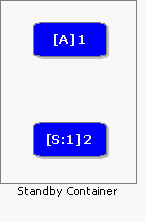
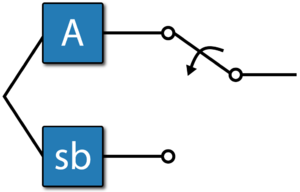
Eqn. 27 can be solved for [math]\displaystyle{ {{t}_{e}} }[/math] and substituted into Eqn.26. Figure "Standby container" illustrates the example as entered in BlockSim using a standby container.

Standby container.

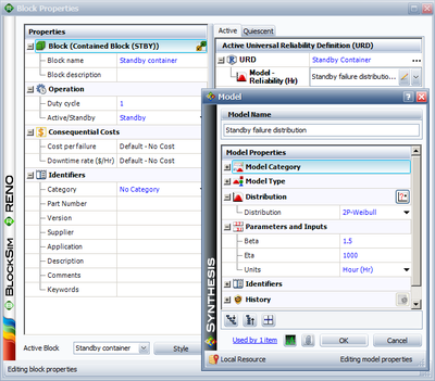
The active and standby blocks are within a container, which is used to specify standby redundancy. Since the standby component has two distributions (active and quiescent), the Block Properties window of the standby block has two pages for specifying each one. Figures "Defining the active failure distribution" and "Defining the quiescent failure distribution" illustrate these pages.

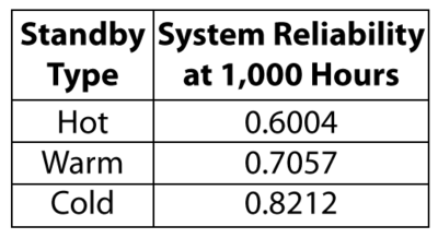
The system reliability results for 1000 hours are given in the following table:

Note that even though the [math]\displaystyle{ \beta }[/math] value for the quiescent distribution is the same as in the active distribution, it is possible that the two can be different. That is, the failure modes present during the quiescent mode could be different from the modes present during the active mode. In that sense, the two distribution types can be different as well (e.g. lognormal when quiescent and Weibull when active).

In many cases when considering standby systems, a switching device may also be present that switches from the failed active component to the standby component. The reliability of the switch can also be incorporated into Eqn.26, as presented in the next section.

BlockSim's System Reliability Equation window returns a single token for the reliability of units in a standby configuration. This is the same as the load sharing case presented in the previous section.

Defining the active failure distribution

Defining the quiescent failure distribution

Reliability of Standby Systems with a Switching Device

In many cases when dealing with standby systems, a switching device is present that will switch to the standby component when the active component fails. Therefore, the failure properties of the switch must also be included in the analysis.

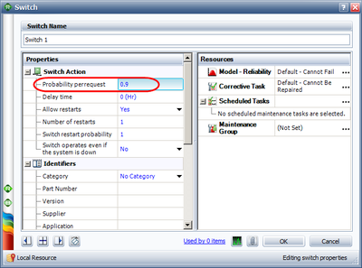
In most cases when the reliability of a switch is to be included in the analysis, two probabilities can be considered. The first and most common one is the probability of the switch performing the action (i.e. switching) when requested to do so. This is called Switch Probability per Request in BlockSim and is expressed as a static probability (e.g. 90%). The second probability is the quiescent reliability of the switch. This is the reliability of the switch as it ages (e.g. the switch might wear out with age due to corrosion, material degradation, etc.). Thus it is possible for the switch to fail before the active component fails. However, a switch failure does not cause the system to fail, but rather causes the system to fail only if the switch is needed and the switch has failed. For example, if the active component does not fail until the mission end time and the switch fails, then the system does not fail. However, if the active component fails and the switch has also failed, then the system cannot be switched to the standby component and it therefore fails.

In analyzing standby components with a switching device, either or both failure probabilities (during the switching or while waiting to switch) can be considered for the switch, since each probability can represent different failure modes. For example, the switch probability per request may represent software-related issues or the probability of detecting the failure of an active component, and the quiescent probability may represent wear-out type failures of the switch.

To illustrate the formulation, consider the previous example that assumes perfect switching. To examine the effects of including an imperfect switch, assume that when the active component fails there is a 90% probability that the switch will switch from the active component to the standby component. In addition, assume that the switch can also fail due to a wear-out failure mode described by a Weibull distribution with [math]\displaystyle{ \beta }[/math] = 1.7 and [math]\displaystyle{ \eta }[/math] = 5000.

Therefore, the reliability of the system at some time, [math]\displaystyle{ t }[/math] , is given by the following equation.

[math]\displaystyle{ \begin{align} R(t)= & {{R}_{1}}(t) \\ & +\underset{0}{\overset{t}{\mathop \int }}\,\{{{f}_{1}}(x)\cdot {{R}_{2;SB}}(x) \\ & \cdot \frac{{{R}_{2;A}}({{t}_{e}}+t-x)}{{{R}_{2;A}}({{t}_{e}})}\cdot {{R}_{SW;Q}}(x)\cdot {{R}_{SW;REQ}}(x)\}dx \end{align} }[/math]

Where:

• [math]\displaystyle{ {{R}_{1}} }[/math] is the reliability of the active component.

• [math]\displaystyle{ {{f}_{1}} }[/math] is the [math]\displaystyle{ pdf }[/math] of the active component.

• [math]\displaystyle{ {{R}_{2;SB}} }[/math] is the reliability of the standby component when in standby mode (quiescent reliability).

• [math]\displaystyle{ {{R}_{2;A}} }[/math] is the reliability of the standby component when in active mode.

• [math]\displaystyle{ {{R}_{SW;Q}} }[/math] is the quiescent reliability of the switch.

• [math]\displaystyle{ {{R}_{SW;REQ}} }[/math] is the switch probability per request.

• [math]\displaystyle{ {{t}_{e}} }[/math] is the equivalent operating time for the standby unit if it had been operating at an active mode.

This problem can be solved in BlockSim by including these probabilities in the container's properties, as shown in Figures "Standby container (switch) failure probabilities while attempting to switch" and "Standby container (switch) failure distribution while waiting to switch". In BlockSim, the standby container is acting as the switch.

Standby container (switch) failure probabilities while attempting to switch

Standby container (switch) failure distribution while waiting to switch

Note that there are additional properties that can be specified in BlockSim for a switch, such as Switch Restart Probability, No. of Restarts and Switch Delay Time. In many applications, the switch is re-tested (or re-cycled) if it fails to switch the first time. In these cases, it might be possible that it switches in the second or third, or [math]\displaystyle{ {{n}^{th}} }[/math] attempt.
The Switch Restart Probability specifies each additional attempt's probability of successfully switching and the Finite Restarts specifies the total number of attempts. Note that the Switch Restart Probability specifies the probability of success of each trial (or attempt). The probability of success of [math]\displaystyle{ n }[/math] consecutive trials is calculated by BlockSim using the binomial distribution and this probability is then incorporated into Eqn.28. The Switch Delay Time property is related to repairable systems and is considered in BlockSim only when using simulation. When using the analytical solution (i.e. for a non-repairable system), this property is ignored.

Solving the analytical solution (as given by Eqn. 28), the following results are obtained.

From the table above, it can be seen that the presence of a switching device has a significant effect on the reliability of a standby system. It is therefore important when modeling standby redundancy to incorporate the switching device reliability properties. It should be noted that this methodology is not the same as treating the switching device as another series component with the standby subsystem. This would be valid only if the failure of the switch resulted in the failure of system (e.g. switch failing open). In Eqn.28, the Switch Probability per Request and quiescent probability are present only in the second term of the equation. Treating these two failure modes as a series configuration with the standby subsystem would imply that they are also present when the active component is functioning (i.e. first term of Eqn.28). This is invalid and would result in the underestimation of the reliability of the system. In other words, these two failure modes become significant only when the active component fails.

As an example, and if we consider the warm standby case, the reliability of the system without the switch is 70.57% at 1000 hours. If the system was modeled so that the switching device was in series with the warm standby subsystem, the result would have been:

[math]\displaystyle{ \begin{align} {{R}_{S}}(1000)= & {{R}_{Standby}}(1000)\cdot {{R}_{sw,Q(1000)}}\cdot {{R}_{sw,req}} \\ = & 0.7057\cdot 0.9372\cdot 0.9 \\ = & 0.5952 \end{align} }[/math]

In the case where a switch failure mode causes the standby subsystem to fail, then this mode can be modeled as an individual block in series with the standby subsystem.

Example 6

Consider a car with four new tires and a full-size spare. Assume the following failure characteristics:

• The tires follow a Weibull distribution with a [math]\displaystyle{ \beta=4 }[/math] and an [math]\displaystyle{ \eta = }[/math] 40,000 miles while on the car due to wear.

• The tires also have a probability of failing due to puncture or other causes. For this, assume a constant rate for this occurrence with a probability of 1 every 50,000 miles.

• When not on the car (i.e. is a spare), a tire's probability of failing also has a Weibull distribution with a [math]\displaystyle{ \beta = }[/math] 2 and [math]\displaystyle{ \eta = }[/math] 120,000 miles.

Assume a mission of 1,000 miles. If a tire fails during this trip, it will be replaced with the spare. However, the spare will not be repaired during the trip. In other words, the trip will continue with the spare on the car and if the spare fails the system will fail. Determine the probability of system failure.

Solution to Example 6

Active failure distribution for tires:

• Due to wear-out, Weibull [math]\displaystyle{ \beta =4 }[/math] and [math]\displaystyle{ \eta =40,000 }[/math] miles.

• Due to random puncture, exponential [math]\displaystyle{ \mu =50,000. }[/math]

• The quiescent failure distribution is a Weibull distribution with [math]\displaystyle{ \beta =2 }[/math] and [math]\displaystyle{ \eta =120,000 }[/math] miles.

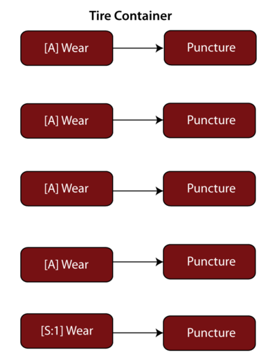
The block diagram for each tire has two blocks in series, one block representing the wear-out mode and the other the random puncture mode, as shown next:

There are five tires, four active and one standby (represented in the diagram by a standby container with a 4-out-of-5 requirement), as shown next:

For the standby Wear block, set the active failure and the quiescent distributions, but for the Puncture block, set only the active puncture distribution (because the tire cannot fail due to puncture while stored). Using BlockSim, the probability of system failure is found to be 0.003 or 0.3%.

Note Regarding Numerical Integration Solutions

Load sharing and standby solutions in BlockSim are performed using numerical integration routines. As with any numerical analysis routine, the solution error depends on the number of iterations performed, the step size chosen and related factors, plus the behavior of the underlying function. By default, BlockSim uses a certain set of preset factors. In general, these defaults are sufficient for most problems. If a higher precision or verification of the precision for a specific problem is required, BlockSim's preset options can be modified and/or the integration error can be assessed using the Integration Parameters... option for each container. For more details, you can refer to the documentation on the Algorithm Setup window in the BlockSim 8 User's help files.